
Videos
a.
Check whether the data provide convincing support for the claim that, on average, male teenager drivers exceed the speed limit by more than do female teenage drivers.
a.
Answer to Problem 18E
The conclusion is that the data provide convincing support for the claim that, on average, male teenager drivers exceed the speed limit by more than do female teenage drivers.
Explanation of Solution
Calculation:
The data are based on the speed limit for male and female drivers.
Step 1:
In this context,
Step 2:
Null hypothesis:
Step 3:
Alternative hypothesis:
Step 4:
Significance level,
It is given that the significance level,
Step 5:
Test statistic:
Step 6:
The assumption for the two-sample t-test:
- The random samples should be collected independently.
- The sample sizes should be large. That is, each sample size is at least 30 or the populations are approximately normally distributed.
It is assumed that the distribution of the speed limit for male and female drivers is normally distributed.
Boxplot:
Software procedure:
Step-by-step procedure to obtain a boxplot using MINITAB software:
- Choose Graphs > Boxplot.
- Under Multiple Y’s, choose Simple.
- In Graph variables, enter the column of Male Driver and Female Driver.
- In Scale, choose Transpose values and categorical scales.
- Click OK in all dialogue boxes.
Output using MINITAB software is given below:
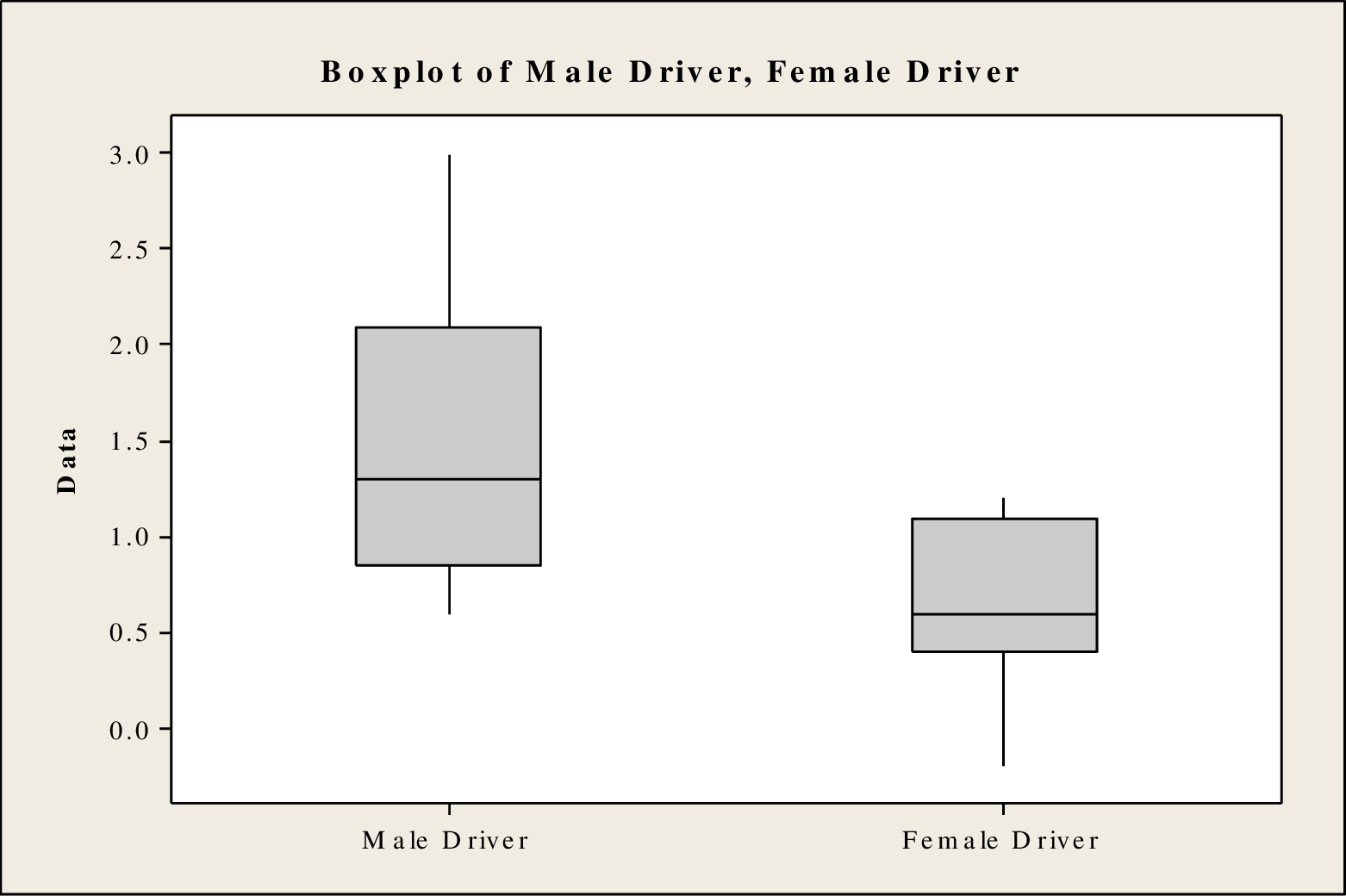
Any lack of symmetric that appears in the boxplot is acceptable for the given sample size because the sample size is larger.
From the boxplot, it is clear that the distribution of the speed limit for male drivers is skewed right and the distribution of the speed limit for female drivers is skewed left. Based on the sample size, the normality condition is satisfied. Morevoer, random samples are collected independently. Therefore, the assumptions are satisfied. It is reasonable to use the data for a two-sample t test.
Step 7:
Test statistic:
Software procedure:
Step-by-step procedure to obtain the P-value and test statistic using MINITAB software:
- Choose Stat > Basic Statistics > 2 sample t.
- Choose Samples in different columns.
- In sample 1, enter the column of Male Driver.
- In sample 2, enter the column of Female Driver.
- Choose Options.
- In Confidence level, enter 95.
- In Alternative, select greater than.
- Click OK in all the dialogue boxes.
Output obtained using MINITAB software is given below:
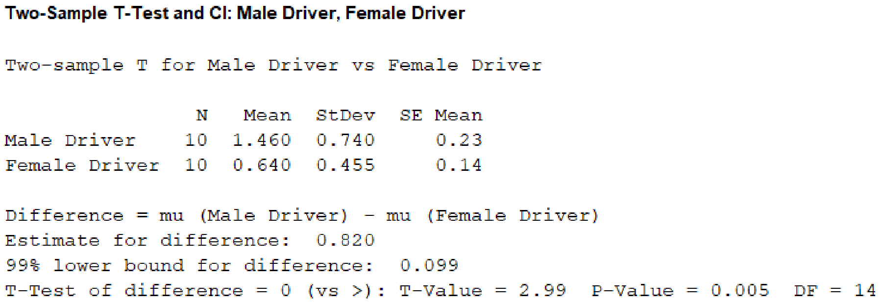
From the given MINITAB output, the value of the test statistic is 2.99.
Step 8:
P-value:
From the MINITAB output, the P-value is 0.005.
Step 9:
Decision rule:
If the
Here, the
That is,
The decision is that the null hypothesis is rejected.
Conclusion:
Hence, the data provide convincing support for the claim that, on average, male teenager drivers exceed the speed limit by more than do female teenage drivers.
b.
(i)
Check whether there is sufficient evidence to conclude that the average number of miles per hour over the speed limit is greater for male drivers with male passengers than it is for male drivers with female passengers.
(ii)
Check whether there is sufficient evidence to conclude that the average number of miles per hour over the speed limit is greater for female drivers with male passengers than it is for female drivers with female passengers.
(iii)
Check whether there is sufficient evidence to conclude that the average number of miles per hour over the speed limit is smaller for male drivers with female passengers than it is for female drivers with male passengers.
b.
Answer to Problem 18E
(i)
The conclusion is that there is sufficient evidence to conclude that the average number of miles per hour over the speed limit is greater for male drivers with male passengers than it is for male drivers with female passengers.
(ii)
The conclusion is that there is sufficient evidence to conclude that the average number of miles per hour over the speed limit is greater for female drivers with male passengers than it is for female drivers with female passengers.
(iii)
The conclusion is that there is sufficient evidence to conclude that the average number of miles per hour over the speed limit is smaller for male drivers with female passengers than it is for female drivers with male passengers.
Explanation of Solution
Calculation:
(i)
Step 1:
In this context,
Step 2:
Null hypothesis:
Step 3:
Alternative hypothesis:
Step 4:
Significance level,
It is given that the significance level
Step 5:
Test statistic:
Step 6:
Assumptions for the two-sample t-test:
- The random samples should be collected independently.
- The sample sizes should be large. That is, each sample size must be at least 30.
Assumption in this particular problem:
- Data are collected independently.
- The sample sizes are large.
Here, both sample sizes are greater than 30.
Therefore, the assumptions are satisfied.
Step 7:
Test statistic:
Software procedure:
Step-by-step procedure to obtain the P-value and test statistic using MINITAB software:
- Choose Stat > Basic Statistics > 2 sample t.
- Choose Summarized data.
- In sample 1, enter Sample size as 40, Mean as 5.2, Standard deviation as 0.8.
- In sample 2, enter Sample size as 40, Mean as 0.3, Standard deviation as 0.8.
- Choose Options.
- In Confidence level, enter 99.
- In Alternative, select greater than.
- Click OK in all the dialogue boxes.
Output obtained using MINITAB software is given below:
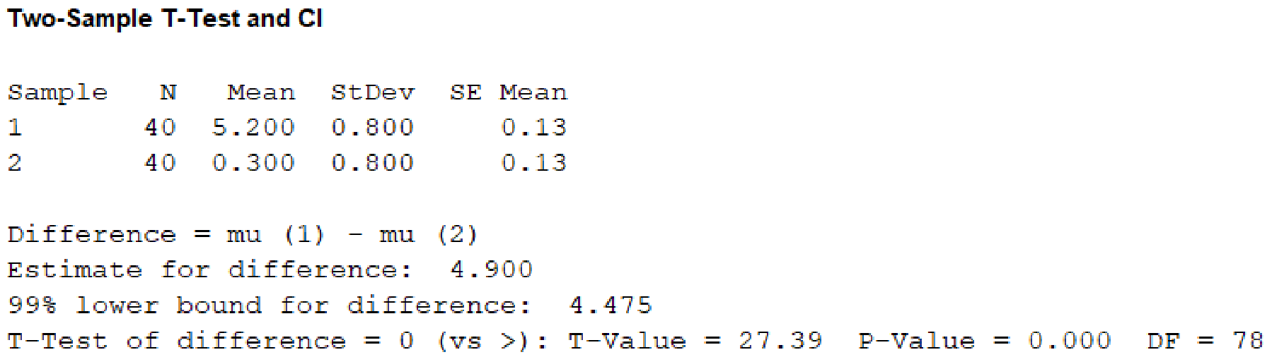
From the given MINITAB output, the value of test statistic is 27.39.
Step 8:
P-value:
From the MINITAB output, the P-value is 0.
Step 9:
Decision rule:
If the
Here, the
That is,
The decision is that the null hypothesis is rejected.
Conclusion:
Hence, there is sufficient evidence to conclude that the average number of miles per hour over the speed limit is greater for male drivers with male passengers than it is for male drivers with female passengers.
(ii)
Step 1:
In this context,
Step 2:
Null hypothesis:
Step 3:
Alternative hypothesis:
Step 4:
Significance level,
It is given that the significance level
Step 5:
Test statistic:
Step 6:
Assumptions for the two-sample t-test:
- The random samples should be collected independently.
- The sample sizes should be large. That is, each sample size must be at least 30.
Assumption in this particular problem:
- Data are collected independently.
- The sample sizes are large.
Here, both sample sizes are greater than 30.
Therefore, the assumptions are satisfied.
Step 7:
Test statistic:
Software procedure:
Step-by-step procedure to obtain the P-value and test statistic using MINITAB software:
- Choose Stat > Basic Statistics > 2 sample t.
- Choose Summarized data.
- In sample 1, enter Sample size as 40, Mean as 2.3, Standard deviation as 0.8.
- In sample 2, enter Sample size as 40, Mean as 0.6, Standard deviation as 0.8.
- Choose Options.
- In Confidence level, enter 99.
- In Alternative, select greater than.
- Click OK in all the dialogue boxes.
Output obtained using MINITAB software is given below:
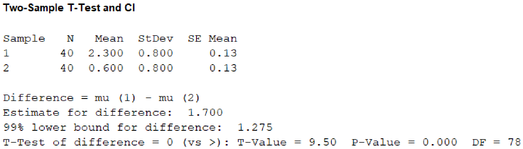
From the given MINITAB output, the value of test statistic is 9.50.
Step 8:
P-value:
From the MINITAB output, the P-value is 0.
Step 9:
Decision rule:
If the
Here, the
That is,
The decision is that the null hypothesis is rejected.
Conclusion:
Hence, there is sufficient evidence to conclude that the average number of miles per hour over the speed limit is greater for female drivers with male passengers than it is for female drivers with female passengers.
(iii)
Step 1:
In this context,
Step 2:
Null hypothesis:
Step 3:
Alternative hypothesis:
Step 4:
Significance level,
It is given that the significance level
Step 5:
Test statistic:
Step 6:
Assumptions for the two-sample t-test:
- The random samples should be collected independently.
- The sample sizes should be large. That is, each sample size must be at least 30.
Assumption in this particular problem:
- Data are collected independently.
- The sample sizes are large.
Here, both sample sizes are greater than 30.
Therefore, the assumptions are satisfied.
Step 7:
Test statistic:
Software procedure:
Step-by-step procedure to obtain the P-value and test statistic using MINITAB software:
- Choose Stat > Basic Statistics > 2 sample t.
- Choose Summarized data.
- In sample 1, enter Sample size as 40, Mean as 0.3, Standard deviation as 0.8.
- In sample 2, enter Sample size as 40, Mean as 2.3, Standard deviation as 0.8.
- Choose Options.
- In Confidence level, enter 99.
- In Alternative, select less than.
- Click OK in all the dialogue boxes.
Output obtained using the MINITAB software is given below:
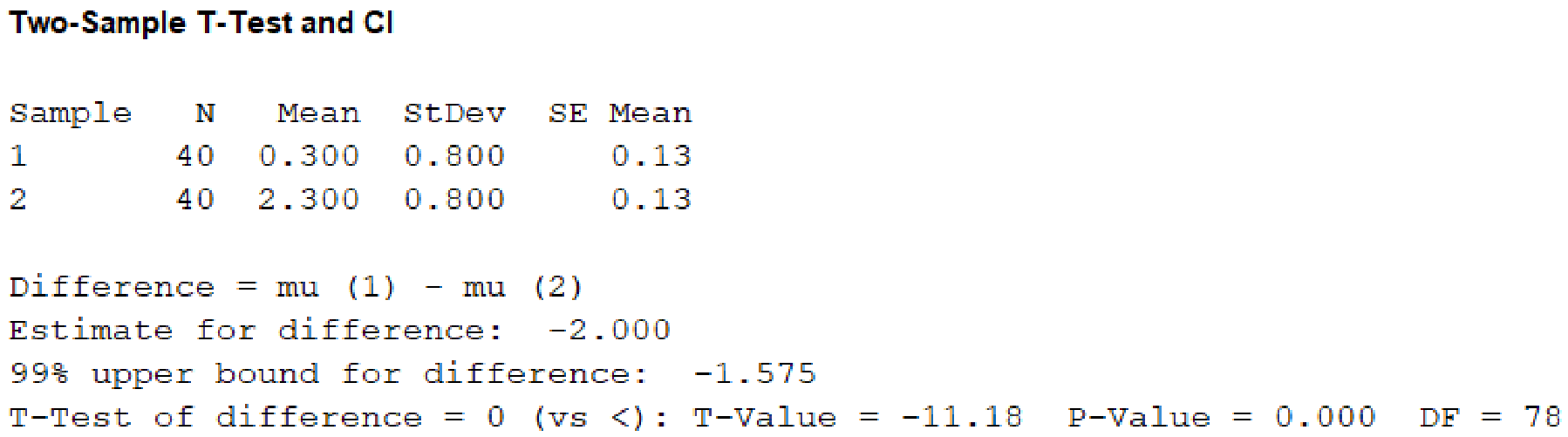
From the given MINITAB output, the value of test statistic is –11.18.
Step 8:
P-value:
From the MINITAB output, the P-value is 0.
Step 9:
Decision rule:
If the
Here, the
That is,
The decision is that the null hypothesis is rejected.
Conclusion:
Hence, there is sufficient evidence to conclude that the average number of miles per hour over the speed limit is smaller for male drivers with female passengers than it is for female drivers with male passengers.
c.
Comment on the effects of gender on teenagers driving with passengers.
c.
Explanation of Solution
Comment:
From the results, it is observed that the average speed limit for male and female drivers are greater with male passengers when compared to the female passengers. The average speed limit for male drivers are lesser with female passengers when compared to the female drivers with male passengers. The average speed limit for male drivers are greater with male passengers when compared to the female drivers with female passengers.
Want to see more full solutions like this?
Chapter 11 Solutions
INTRO.TO STATS.+DATA ANALYS. W/WEBASSI


- The following data were obtained from an independent-measures study comparing three treatment conditions. Treatment I II III 4 3 8 N = 12 3 1 4 G = 48 5 3 6 ΣX2 = 238 4 1 6 M = 4 M = 2 M = 6 T = 16 T = 8 T = 24 SS =2 SS = 4 SS = 8 A) Use an ANOVA with alpha = .05 to determine whether there are any significant differences among the three treatment means. Follow the four-step procedure of hypothesis testing. B) Calculate the eta squared to measure the effect size. C) Report your results of one-way ANOVA analysis and the effect size in APA format. D) conduct a post hoc analysis with Tukey’s HSDarrow_forwardA Canadian study measuring depression level in teens (as reported in the Journal of Adolescence, vol. 25, 2002) randomly sampled 112 male teens and 101 female teens, and scored them on a common depression scale (higher score representing more depression). The researchers suspected that the mean depression score for male teens is higher than for female teens, and wanted to check whether data would support this hypothesis. If μ1 and μ2 represent the mean depression score for male teens and female teens respectively, which of the following is an appropriate pair of hypotheses in this case? Check all that apply.arrow_forwardFollowing is the rating of marketing aggressivity (X) and sales performance (Y) of 8 sales staffs in Glovis Co in the past year: Table Attached Question: What is the hypothesis of the study?arrow_forward
- On snow-covered roads, winter tires enable a car to stop in a shorter distance than if summer tires were installed. In terms of the additive model for one-way ANOVA, and for an experiment in which the mean stopping distances on a snow-covered road are measured for each of four brands of winter tires. If the data are as shown in Sheet 48, what conclusion would be reached at the 0.01 level of significance? Shett 48 Supplier A 517 484 463 452 502 447 481 500 485 566 Supplier B 479 499 488 430 482 457 424 488 526 455 Supplier C 435 443 480 465 435 430 465 514 463 510 Supplier D 526 537 443 505 468 533 481 477 490 470 Select one: a) p-value = 0.28 greater than 0.05, the average distance is different for at list two tires b) F stat = 1.86, F crit = 4.38, not enough evidence to claim that the average distance is different for at list two tires c) F ratio = 4.38, not enough evidence to claim that the average distance is different for at list two tires d) F stat = 0.68, F…arrow_forwardA sample of men and women who had passed their driver's test either the first time or the second time were surveyed, with the following results: Results of the driving testGender First time Second timeMen 126 211Women 135 178a) Do these data suggest that there is a relationship between gender and the passing of their driver’s test from which the present sample was drawn? Let alpha=.05arrow_forwardFollowing are the protein contents measured in two types of species:Species 1: 0.72 1.12 0.81 0.89 0.72 0.81 1.01 0.75 0.83Species 2: 1.21 0.93 0.80 1.12 1.22 0.94 0.87 i) Assuming normality, test the hypothesis that the two species have the sameaverage protein contents by using 5-step hypothesis testing procedure at 5 %level of significance, and using the critical values approach.ii) Calculate the p-value of this test and make decision.iii) Write down the standard error of this test and calculate its numerical value ?arrow_forward
- Independent random samples of 32 people living on the west side of a city and 30 people living on the east side of a city were taken to determine if the income levels of west side residents are significantly different from the income levels of east side residents. Given the testing statistics below, determine if the data provides sufficient evidence to conclude that the income levels of west side residents are significantly different from the income levels of east side residents, at the 2% significance level. H0:μw=μeHa:μw≠μe t0=2.364 t0.01=±2.099 Select the correct answer below: No; the test statistic is not between the critical values. No; the test statistic is between the critical values. Yes; the test statistic is not between the critical values. Yes; the test statistic is between the critical values.arrow_forwardIn a clinical trial, 17 out of 900 patients taking a prescription drug complaint of flu like symptoms. Suppose that it is known that 1.3% of the patients taking competing drugs complain of flu like symptoms. Is there sufficient evidence to conclude that more than 1.3% of the drugs user experience food like symptoms as a side effect at the 0.01 level of significance? what are the normal and alternative hypothesis?arrow_forwardThe following are the laboratory results in hemoglobin of 10 male (X1) and 10 female(X2) patients. Test the null hypothesis that there is no significant difference between the hemoglobin of male and female patients. Use the t -test at 0.05 level of significance. X1 14 18 17 16 4 14 12 10 9 17 X2 12 9 11 5 10 3 7 2 6 13 Null and Alternative Hypothesis Level of significance Critical value T-test value P-value Decision Conclusionarrow_forward
- In its January 25, 2012, issue, the Journal of the American Medical Association reported on the effects of overconsumption of low, normal, and high protein diets on weight gain, energy expenditure, and body composition. Researchers conducted a single blind, randomized controlled trial of 25 U.S. adults. The subjects were healthy, weight-stable, male and female volunteers, aged 18 to 35 years. All subjects consumed a weight-stabilizing diet for 13 to 25 days. Afterwards, the researchers randomly assigned participants to diets containing various percentages of energy from protein: 5% (low protein), 15% (normal protein), or 25% (high protein). The subjects were not aware of the specific protein level diet to which they were assigned. On these diets the researchers overfed the participants during the last 8 weeks of their 10 to 12 week stay in the inpatient metabolic unit. The goal was to investigate the effect of overconsumption of protein on weight gain, energy expenditure, and body…arrow_forwardFor a special pre-New Year's Eve show, a radio station personality has invited a small panel of prominent local citizens to help demonstrate to listeners the adverse effect of alcohol on reaction time, thus drinking an alcohol increases reaction time. The reaction times (in seconds) before and after consuming four drinks are in Sheet 11. Test a hypothesis to see if the showman claim is supported by the given data (use alpha=0.01 significance level). Sheet 11 Subject Before After 1 0,32 0,39 2 0,39 0,44 3 0,36 0,49 4 0,41 0,53 5 0,37 0,46 6 0,35 0,39 7 0,37 0,49 8 0,37 0,52 9 0,32 0,43 10 0,39 0,45 11 0,39 0,39 12 0,41 0,49 13 0,32 0,48 14 0,38 0,48 15 0,34 0,4 16 0,35 0,52 Select one: a. The alternative hypothesis that the reaction time before consuming alcohol is less than after is not accepted as the p-value= 0.0000 is less than alpha=0.005 b. The Null hypothesis that the reaction time before consuming alcohol is less than after is rejected…arrow_forwardListed below are paired data consisting of waist size in centimeters and Body Mass Index BMI from a random sample of 20 adult men selected from the population. At the a = 0.05 significance level, test the claim that there is positive linear correlation between waist size and Body Mass Indices in adult men, by answering questions a. thru e. below. That is, test the claim: ρ>0 This uses a Null Hypothesis of ρ =0 and an Alternative Hypothesis of ρ>0 WAIST BMI 120.4 33.3 107.8 28.0 120.3 45.4 97.2 28.4 95.1 25.9 112.0 31.1 78.0 20.1 103.5 32.7 89.7 25.8 112.0 36.5 95.0 25.8 115.3 34.5 118.8 37.4 92.6 26.1 75.5 19.3 101.8 29.9 92.5 27.4 100.8 31.4 82.8 21.0 92.9 28.5 a. What is the linear correlation coefficient r = ___________________________ b. What is the P-Value…arrow_forward
 MATLAB: An Introduction with ApplicationsStatisticsISBN:9781119256830Author:Amos GilatPublisher:John Wiley & Sons Inc
 Probability and Statistics for Engineering and th...StatisticsISBN:9781305251809Author:Jay L. DevorePublisher:Cengage Learning
 Statistics for The Behavioral Sciences (MindTap C...StatisticsISBN:9781305504912Author:Frederick J Gravetter, Larry B. WallnauPublisher:Cengage Learning
 Elementary Statistics: Picturing the World (7th E...StatisticsISBN:9780134683416Author:Ron Larson, Betsy FarberPublisher:PEARSON
 The Basic Practice of StatisticsStatisticsISBN:9781319042578Author:David S. Moore, William I. Notz, Michael A. FlignerPublisher:W. H. Freeman
 Introduction to the Practice of StatisticsStatisticsISBN:9781319013387Author:David S. Moore, George P. McCabe, Bruce A. CraigPublisher:W. H. Freeman