
Videos
The accompanying data resulted from an experiment to investigate whether yield from a certain chemical process depended either on the formulation of a particular input or on mixer speed.
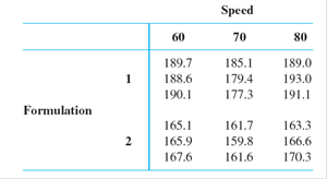
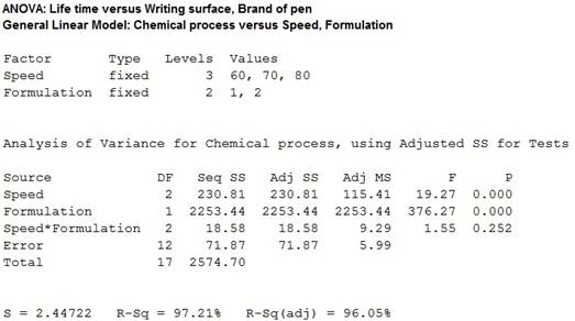
A statistical computer package gave SS(Form) = 2253.44, SS(Speed) = 230.81, SS(Form*Speed) = 18.58, and SSE = 71.87.
a. Does there appear to be interaction between the factors?
b. Does yield appear to depend on either formulation or speed?
c. Calculate estimates of the main effects.
d. The fitted values are
e. Construct a normal probability plot from the residuals given in part (d). Do the ϵijk’s appear to be
a.
Identify whether there is a significant effect from interaction between speed and formulation.
Answer to Problem 18E
There is no sufficient evidence to conclude that there is an effect of interaction between mix speed and formulation on the chemical process.
Explanation of Solution
Given info:
An experiment was carried out to test the effect of formulation and speed on the chemical press. The formulation has two levels and speed has three levels.
The sum of squares due to formulation is 2,253.44, sum of squares due to speed is 230.81, sum of squares due to error is 71.87, sum of squares due to interaction between formulation and speed is 18.58.
Calculation:
Testing the Hypothesis:
Null hypothesis:
That is, the interaction effect between mix speed and formulation has no significant effect on chemical process.
Alternative hypothesis:
That is, the interaction effect between mix speed and formulation has no significant effect on chemical process.
Test statistic:
Software procedure:
Step by step procedure to find the test statistic using Minitab is given below:
- Choose Stat > ANOVA > General Linear Model.
- In Responses, enter the column of Chemical process.
- In Model, enter the column of Speed, Formulation, Speed*Formulation.
- In Results, choose “Analysis of variance table”.
- Click OK in all dialog boxes.
Output obtained from MINITAB is given below:
Conclusion:
Interaction effect of AB:
The P- value for the interaction effect AB is 0.252 and the level of significance is 0.01.
The P- value is lesser than the level of significance.
That is,
Thus, the null hypothesis is not rejected,
Hence, there is no sufficient evidence to conclude that there is an effect of interaction between mix speed and formulation on the chemical process.
b.
Identify whether the yield of the chemical process depends on speed or formulation.
Answer to Problem 18E
The yield of a chemical process depends on both speed and formulation.
Explanation of Solution
From the MINITAB output obtained in part (a), the following can be observed.
For Main effect of factor A speed:
The P- value for the factor A (speed) is 0.000 and the level of significance is 0.01.
The P- value is lesser than the level of significance.
That is,.
Thus, the null hypothesis is rejected,
Hence, there is sufficient evidence to conclude that there is an effect of speed on the yield of chemical process.
For Main effect of factor B formulation:
The P- value for the factor B (formulation) is 0.000 and the level of significance is 0.01.
The P- value is lesser than the level of significance.
That is,
Thus, the null hypothesis is rejected,
Hence, there is sufficient evidence to conclude that there is an effect of formulation on the yield of chemical process.
c.
Find the estimates for the main effects.
Explanation of Solution
Calculation:
Where,
Overall mean effect:
Mean due to the first level of factor A:
Mean due to the second level of factor A:
Main effect of factor A:
At first level:
At second level:
Mean due to the first level of factor B:
Mean due to the second level of factor B:
Mean due to the third level of factor B
Main effect of factor B:
d.
Verify whether the calculated residuals are equal to the given residual values.
Explanation of Solution
Calculation:
The interaction effect for the first level of factor A and the first level of factor B
The interaction effect for the first level of factor A and the second level of factor B
The interaction effect for the first level of factor A and the third level of factor B
Similarly, the remaining values are given below:
| S. No | Values |
| 1 | |
| 2 | |
| 3 | |
| 4 | |
| 5 | |
| 6 |
The fitted values are calculated by using the formula:
Where,
i represents the levels of factor A.
j represents the levels of factor B.
k represents the observation.
The predicted value when
Similarly, the other fitted values are calculated, the table shows the fitted values:
| S. No | 1 | 2 | 3 | 4 | 5 | 6 | 7 | 8 | 9 |
| Fitted values | 189.47 | 189.47 | 189.47 | 166.20 | 166.20 | 166.20 | 180.60 | 180.60 | 180.60 |
| S. No | 10 | 11 | 12 | 13 | 14 | 15 | 16 | 17 | 18 |
| Fitted values | 161.03 | 161.03 | 161.03 | 191.03 | 191.03 | 191.03 | 166.73 | 166.73 | 166.73 |
The residuals values are calculated by using the formula:
The table shows below gives the residuals for each observation:
| S. No |
Observed |
Fitted values | |
| 1 | 189.7 | 189.47 | 0.23 |
| 2 | 188.6 | 189.47 | –0.87 |
| 3 | 190.1 | 189.47 | 0.63 |
| 4 | 165.1 | 166.20 | –1.1 |
| 5 | 165.9 | 166.20 | –0.3 |
| 6 | 167.6 | 166.20 | 1.4 |
| 7 | 185.1 | 180.60 | 4.5 |
| 8 | 179.4 | 180.60 | –1.2 |
| 9 | 177.3 | 180.60 | –3.3 |
| 10 | 161.7 | 161.03 | 0.67 |
| 11 | 159.8 | 161.03 | –1.23 |
| 12 | 161.6 | 161.03 | 0.57 |
| 13 | 189 | 191.03 | –2.03 |
| 14 | 193 | 191.03 | 1.97 |
| 15 | 191.1 | 191.03 | 0.07 |
| 16 | 163.3 | 166.73 | –3.43 |
| 17 | 166.6 | 166.73 | –0.13 |
| 18 | 170.3 | 166.73 | 3.57 |
Hence, the calculated residuals values are equal to given residual values.
e.
Construct a normal probability plot for the residuals obtained in part (d).
Identify whether the residuals are normally distributed.
Answer to Problem 18E
The normal probability of residuals is given below:
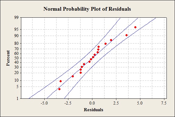
The residuals are normally distributed.
Explanation of Solution
Calculation:
Normal probability plot of residuals:
Software procedure:
Step-by-step procedure to construct a normal probability plot of residuals is given below:
- Click on Graph>Probability plot>Single.
- Click OK.
- Under Graph variables, select the column containing the residual values.
- Click on Distribution and selection Normal.
- Click OK.
Interpretation:
The normal probability plot of residuals suggests that the residuals are normally distributed because the residuals fall approximately on a straight line.
Want to see more full solutions like this?
Chapter 11 Solutions
Bundle: Probability And Statistics For Engineering And The Sciences, 9th + Webassign, Single-term Printed Access Card


- what would a positive association mean betwwen these two variables? briefly explain why a poaitive relationship might make sense in.this context.arrow_forwardHere is a dataset containing plant growth measurements of plants grown in solutions of commonly-found chemicals in roadway runoff.Phragmites australis, a fast-growing non-native grass common to roadsides and disturbed wetlands of Tidewater Virginia, was grown in a greenhouse and watered with either: Distilled water (control); A weak petroleum solution (representing standard roadway runoff); Sodium chloride solution; Magnesium chloride solution; De-icing brine (50% sodium chloride and 50% magnesium chloride).Twenty grass preparations were used for each solution, and total growth (in cm) was recorded after watering every other day for 40 days.-Perform the correct statistical test to determine the p-value.-Report your answer rounded to four decimal places.-You should use formulas, functions, and the Data Analysis ToolPak in MS Excel to avoid additive rounding errors. Here are some useful functions: =t.test(array1,array2,tails,type) Produces a p-value for any…arrow_forwardWhich model—the one for parliaments or the one for ministries (or cabinets)—presented in the article has the greater explanatory power? How can you tell?arrow_forward
- Which of the independent variables retains the strongest association with the number of children a respondent has when all other variables in the model are controlled?arrow_forwardUse this data and create a model that estimates a student's giving rate as an alumni based on the three parameters provided. If a class has a graduation rate of 74, the % of classes under 20 student equal to 55, and a Student=Faculty Ratio of 19, what should we expect our Alumni Giving Rate to be? (Enter a whole number) University Graduation Rate % of Classes Under 20 Student-Faculty Ratio Alumni Giving Rate Boston College 85 39 13 25 Brandeis University 79 68 8 33 Brown University 93 60 8 40 California Institute of Technology 85 65 3 46 Carnegie Mellon University 75 67 10 28 Case Western Reserve Univ. 72 52 8 31 College of William and Mary 89 45 12 27 Columbia University 90 69 7 31 Cornell University 91 72 13 35 Dartmouth College 94 61 10 53 Duke University 92 68 8 45 Emory University 84 65 7 37 Georgetown University 91 54 10 29 Harvard University 97 73 8 46 Johns Hopkins University 89 64 9 27 Lehigh University 81 55 11 40 Massachusetts Inst.…arrow_forwardHere are some data I found on the enzyme activity of mannose-6-phosphate isomerase (MPI) and MPI genotypes in the amphipod crustacean Platorchestia platensis. Because I didn't know whether sex also affected MPI activity, I separated the amphipods by sex. F and S stand for fast and slow respectively, and have to do with electrophoretic mobility on an agarose gel. FF, FS, and SS then reflect genotypes with FS being the heterozygote. Consider the numbers to be activity units. Analysis these data with the appropriate two-way ANOVA and state your conclusions below. Genotype Female Male FF 2.838 1.884 4.216 2.283 2.889 4.939 4.198 3.486 FS 3.55 2.396 4.556 2.956 3.087 3.105 1.943 2.649 SS 3.62 2.801 3.079 3.421 3.586 4.275 2.669 3.11 I use excel for this questionarrow_forward
- A well-known multinational FMCG produces more than fifty products and sells them in themarket. Out of fifty products one is mineral water for drinking purpose and supplies differentsize pack bottles in the market. Product manager observed that, during hot days the sale of wateris more as compared to the normal days. He started the collection of data of weekly sale of waterand the average weekly temperature.Product manager was interested in developing a relationship between sales and temperature;therefore, he discussed and shared the following data with you. sales 7577696379807770738772738080698477727481 temperature 3236313134293235283130312935362832333233 Sale is in thousand liters and temperature is in degree Celsius. Data is Normally distributedYou are required to determine the following information for some concrete decision: a. Determine the statistical relationship between temperature and sale of water andinterpret.b. How much change in sales if the temperature…arrow_forwardA paper investigated the driving behavior of teenagers by observing their vehicles as they left a high school parking lot and then again at a site approximately 1 2 mile from the school. Assume that it is reasonable to regard the teen drivers in this study as representative of the population of teen drivers. Amount by Which Speed Limit Was Exceeded MaleDriver FemaleDriver 1.2 -0.1 1.4 0.4 0.9 1.1 2.1 0.7 0.7 1.1 1.3 1.2 3 0.1 1.3 0.9 0.6 0.5 2.1 0.5 (a) Use a .01 level of significance for any hypothesis tests. Data consistent with summary quantities appearing in the paper are given in the table. The measurements represent the difference between the observed vehicle speed and the posted speed limit (in miles per hour) for a sample of male teenage drivers and a sample of female teenage drivers. (Use μmales − μfemales.Round your test statistic to two decimal places. Round your degrees of freedom down to the nearest whole number. Round your p-value to…arrow_forwardA researcher is interested in testing the relationship between smoking and BMI (kg/m2) in adults aged 30-45. In order to test this association, the researcher divides smoking into currently more than a pack a day, currently less than a pack a day, and never smokers. The following table represents the BMIs for each participant enrolled by their respective smoking category. Current Smoker (≥1pack/day) Current Smoker (<1 pack/day Never Smoked 26.7 29.4 22.1 29.4 28.6 30.4 24.3 27.4 21.3 28.4 23.2 26.4 21.6 20.1 19.7 27.4 20.6 19.8 26.8 19.7 21.6 36.4 19.6 22.3 31.5 21.6 24.3 27.4 21.5 *Continue as though all assumptions for ANOVA are met. A) Calculate the MSW and MSB for the data represented above. B) Carry out a formal test for a one-way analysis of variance among the groups and interpret your results.arrow_forward
- A paper investigated the driving behavior of teenagers by observing their vehicles as they left a high school parking lot and then again at a site approximately 1 2 mile from the school. Assume that it is reasonable to regard the teen drivers in this study as representative of the population of teen drivers. Amount by Which Speed Limit Was Exceeded MaleDriver FemaleDriver 1.3 -0.1 1.3 0.4 0.9 1.1 2.1 0.7 0.7 1.1 1.3 1.2 3 0.1 1.3 0.9 0.6 0.5 2.1 0.5 (a) Use a .01 level of significance for any hypothesis tests. Data consistent with summary quantities appearing in the paper are given in the table. The measurements represent the difference between the observed vehicle speed and the posted speed limit (in miles per hour) for a sample of male teenage drivers and a sample of female teenage drivers. (Use μmales − μfemales.Round your test statistic to two decimal places. Round your degrees of freedom down to the nearest whole number. Round your p-value to…arrow_forwardThe accompanying data file contains 40 observations on the response variable y along with the predictor variables x1 and x2. Use the holdout method to compare the predictability of the linear model with the exponential model using the first 30 observations for training and the remaining 10 observations for validation. y x1 x2 533.86 20 30 104.84 15 20 64.89 20 23 159.61 16 21 43.06 13 16 4.27 13 13 736.56 15 30 64.89 20 23 10.64 20 22 76.90 18 20 4.89 11 13 80.90 11 16 224.17 12 19 45.75 16 25 8.13 17 17 319.97 13 30 48.61 19 25 564.67 12 27 111.87 11 25 152.39 13 24 13.34 18 14 28.80 15 22 37.56 13 15 105.62 17 26 44.05 18 21 451.65 17 28 10.34 18 21 32.70 12 13 19.21 14 12 14.02 15 16 2.45 16 12 2.48 20 15 50.34 17 21 29.31 17 20 33.75 16 12 196.28 17 29 943.12 13 30 7.25 10 12 89.73 15 25 32.91 12 18 1. Use the training set to estimate Models 1 and 2. Note: Negative values should be indicated by a…arrow_forwardb) What are the three models proposed as extensions of the GARCH model? Describe their advantages over the GARCH.arrow_forward
 MATLAB: An Introduction with ApplicationsStatisticsISBN:9781119256830Author:Amos GilatPublisher:John Wiley & Sons Inc
 Probability and Statistics for Engineering and th...StatisticsISBN:9781305251809Author:Jay L. DevorePublisher:Cengage Learning
 Statistics for The Behavioral Sciences (MindTap C...StatisticsISBN:9781305504912Author:Frederick J Gravetter, Larry B. WallnauPublisher:Cengage Learning
 Elementary Statistics: Picturing the World (7th E...StatisticsISBN:9780134683416Author:Ron Larson, Betsy FarberPublisher:PEARSON
 The Basic Practice of StatisticsStatisticsISBN:9781319042578Author:David S. Moore, William I. Notz, Michael A. FlignerPublisher:W. H. Freeman
 Introduction to the Practice of StatisticsStatisticsISBN:9781319013387Author:David S. Moore, George P. McCabe, Bruce A. CraigPublisher:W. H. Freeman