An Introduction to Statistical Methods and Data Analysis
7th Edition
ISBN: 9781305269477
Author: R. Lyman Ott, Micheal T. Longnecker
Publisher: Cengage Learning
expand_more
expand_more
format_list_bulleted
Videos
Textbook Question
Chapter 11.9, Problem 9E
A manufacturer of cases for sound equipment requires that holes be drilled for metal screws. The drill bits wear out and must be replaced; there is expense not only in the cost of the bits but also in the cost of lost production. Engineers varied the rotation speed of the drill and measured the lifetime y (thousands of holes drilled) of four bits at each of five speeds x. The data were:
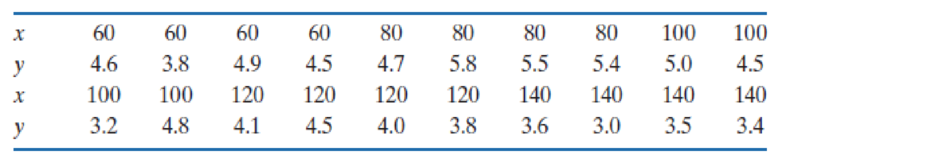
- a. Create a
scatterplot of the data. Does there appear to be a relation? Does it appear to be linear? - b. Is there any evident outlier? If so, does it have high influence?
Expert Solution & Answer
Want to see the full answer?
Check out a sample textbook solution
Students have asked these similar questions
The period T of a pendulum is measured for pendulums of several different lengths L. Based on the following data, does T appear to be a linearfunction of L?
L (cm)
20
30
40
50
T (s)
0.9
1.1
1.27
1.42
The following table shows the annual expenditures, in dollars, per customer unit for residential landline phone services and cellular phone services in the United States in the given year.†
Year
Landline
Cell
2004
592
378
2006
542
524
2008
467
643
2010
401
760
Calculate the regression line for each type of service. (Let t be the time in years since 2004, L be the operating revenue of landline phone services and C be the expenditure of cellular services. Round your regression parameters to two decimal places.)
L(t) =
C(t) =
Determine the expenditure level at which the two lines cross. Round your answer for the expenditure level to one decimal place. million dollars
In a simple ridge regression model, if the (x, y) pairs (0, 1) and (1, 0) yield the same error factor (E or e) of value 2, which of the following may be (closest) used for the regularization parameter λ? a) λ = 0.0
b)λ = 0.5
c)λ = 1.0
d)λ = 1.5
Chapter 11 Solutions
An Introduction to Statistical Methods and Data Analysis
Ch. 11.9 - Prob. 1ECh. 11.9 - Refer to Exercise 11.1.
Plot the equation in the...Ch. 11.9 - Use the data given here to answer the following...Ch. 11.9 - Prob. 4ECh. 11.9 - Use the output from Minitab for these data to...Ch. 11.9 - A food processor was receiving complaints from its...Ch. 11.9 - An online retailer needs to manage the amount of...Ch. 11.9 - A manufacturer of cases for sound equipment...Ch. 11.9 - Refer to the data of Exercise 11.7. a. Calculate a...Ch. 11.9 - Refer to the data of Exercise 11.8.
Calculate a...
Ch. 11.9 - Refer to the data of Exercise 11.8.
Calculate a...Ch. 11.9 - Athletes are constantly seeking measures of the...Ch. 11.9 - A firm that prints automobile bumper stickers...Ch. 11.9 - A chemist is interested in determining the weight...Ch. 11.9 - Refer to Exercise 11.22 to complete the following....Ch. 11.9 - Prob. 40ECh. 11.9 - A survey of MBA, graduates of a business school...Ch. 11.9 - Refer to the data in Exercise 11.44.
Determine the...Ch. 11.9 - There has been an increasing emphasis in recent...Ch. 11.9 - An air conditioning company responds to calls...Ch. 11.9 - Refer to Exercise 11.61. a. Calculate the...Ch. 11.9 - Refer to Exercise 11.61.
Test for lack of fit for...Ch. 11.9 - Refer to Exercise 11.61.
Compute the standard...Ch. 11.9 - Prob. 93SE
Knowledge Booster


Learn more about
Need a deep-dive on the concept behind this application? Look no further. Learn more about this topic, statistics and related others by exploring similar questions and additional content below.Similar questions
- A stamped sheet steel plate is shown in Figure 164. Compute dimensions AF to 3 decimal places. All dimensions are in inches. A=_B=_C=_D=_E=_F=_arrow_forwardThe tables for Exercises 15 and 16 give the position of the zero graduation on the vernier scale in reference to the main scale and the vernier scale graduation that coincides with a main scale graduation. Determine the vernier caliper settings. The answer to the first part of Exercise 15 is givenarrow_forwarduse the map in Figure 11.2. a Find the grid section of Taylor Hall. b. What is located in section 3B?arrow_forward
- Find the Laplace ranform of y(t)arrow_forwardCalculate the coefficient of skewness from the data as follows. Hours No. of Tubes 300-400 14 400-500 46 500-600 58 600-700 76 700-800 68 800-900 62 900-1000 48 1000-1100 22 1100-1200 6arrow_forward6) part 4. Generate a abo plot for the asteroid data.arrow_forward
- Find the value of m, b, and A so that f fits the data.arrow_forwardThe amount of time a student devotes to class attendance and revision: and the grade obtained are assumed to be linearly related. In a small class of 15 students, the following results were obtained for this linear relationship. Y = 30 +2.50.Y (0.55) (2.96) R'= 0.85 The standard errors are in parenthesis. a,Test the hypothesis that the intereept and slope are individually equal to zero (0) at the S% level of signiticance. (b) Construct n 95% conlidence interval for the true slope. (c)Compute the elasticity of grades with respect to time input and interpret your results. (d) Interpret your R' and explain how it relates to the slope of the regression line. (e) From the results and your answers in (a) to (d), does time input into class attendance and revision really influence the final grade?arrow_forwardUse the sample data given in tablex 1 2 3 4 5y 3 4 1 2 1a) To Write the regression equation ̂y=mx+bb) Plot the regression equation and the scatter diagram on the same grapharrow_forward
- The grades of a class of 9 students on a midterm report (x) and on the final examination (y) are as follows: (10) (x) 70 55 72 72 81 94 96 99 67 (y) 80 67 78 34 47 85 99 99 68 a. Find the equation of the regression line. b. Estimate the final examination grade of a student who received a grade of 85 on the midterm report but was ill at the time of the final examination. c. Compute the standard error of estimate.yxS.arrow_forwardJóhannes plans to examine the salary of a middle manager in a large company. He collects data on salaries and how long they have been employed as middle managers with the aim of creating a model that can predict salaries with work experience. Jóhannes has data from 20 randomly selected middle managers who range from being new to the job to having 12 years of work experience. Jóhannes started by drawing the data and sees that the relationship is linear. He also calculates some light sizes that can be seen below: Convert Average Standard deviation Salary 761041 238473 Job experience 5,65 3,71 He also calculated the correlation coefficient between wages and work experience and obtained a r = 0.82. a) Find an equal regression line for Jóhannes's modelb) What is the explanatory power of the model and what does it tell us?c) How much does a middle manager's salary increase in five years according to the model?d) Use the model to predict the salary of a middle manager with 20 years…arrow_forwardWhich of the following is the most appropriate equation to model the data? ŷ = 1.1x + 1.467 ŷ = 1.467x + 1.1 ŷ = 1.1(1.467)x ŷ = 1.467(1.1)xarrow_forward
arrow_back_ios
arrow_forward_ios
Recommended textbooks for you
 Mathematics For Machine TechnologyAdvanced MathISBN:9781337798310Author:Peterson, John.Publisher:Cengage Learning,
 Trigonometry (MindTap Course List)TrigonometryISBN:9781337278461Author:Ron LarsonPublisher:Cengage Learning
 Algebra & Trigonometry with Analytic GeometryAlgebraISBN:9781133382119Author:SwokowskiPublisher:Cengage
Mathematics For Machine Technology
Advanced Math
ISBN:9781337798310
Author:Peterson, John.
Publisher:Cengage Learning,
Trigonometry (MindTap Course List)
Trigonometry
ISBN:9781337278461
Author:Ron Larson
Publisher:Cengage Learning
Algebra & Trigonometry with Analytic Geometry
Algebra
ISBN:9781133382119
Author:Swokowski
Publisher:Cengage
Chain Rule dy:dx = dy:du*du:dx; Author: Robert Cappetta;https://www.youtube.com/watch?v=IUYniALwbHs;License: Standard YouTube License, CC-BY
CHAIN RULE Part 1; Author: Btech Maths Hub;https://www.youtube.com/watch?v=TIAw6AJ_5Po;License: Standard YouTube License, CC-BY