Chapter 12, Problem 22E

(a)

To determine

To find: The fitted data and the residuals. Also, generate the scatterplot of the residuals versus the group variable and check whether the residuals are symmetrically scattered below and above the zero or not and also check if there are any outliers.

Answer to Problem 22E

Solution: The residuals of the provided data is scattered symmetrically above and below the zero and there is no extreme outlier.

Explanation of Solution

Given: The data provided in the Facebook friends study as,

Friends	Participant	Score
102	1	3.8
102	2	3.6
102	3	3.2
102	4	2.4
102	5	4.8
102	6	3.0
102	7	4.2
102	8	3.6
102	9	3.2
102	10	3.0
102	11	4.8
102	12	3.4
102	13	4.8
102	14	3.0
102	15	4.6
102	16	2.8
102	17	6.0
102	18	2.8
102	19	5.2
102	20	3.2
102	21	4.2
102	22	2.2
102	23	5.0
102	24	4.8
302	25	5.0
302	26	5.2
302	27	5.6
302	28	2.6
302	29	3.8
302	30	4.8
302	31	5.6
302	32	4.8
302	33	6.4
302	34	4.8
302	35	4.4
302	36	6.0
302	37	3.8
302	38	4.8
302	39	4.6
302	40	6.0
302	41	5.0
302	42	3.0
302	43	4.4
302	44	5.4
302	45	5.4
302	46	4.6
302	47	5.6
302	48	5.8
302	49	4.2
302	50	4.8
302	51	5.0
302	52	5.2
302	53	4.2
302	54	5.0
302	55	5.8
302	56	5.6
302	57	3.8
502	58	4.6
502	59	4.0
502	60	4.8
502	61	3.0
502	62	2.0
502	63	5.8
502	64	5.6
502	65	4.4
502	66	4.4
502	67	5.6
502	68	4.6
502	69	5.6
502	70	3.0
502	71	5.6
502	72	3.6
502	73	6.8
502	74	3.2
502	75	4.8
502	76	4.6
502	77	5.4
502	78	4.8
502	79	4.8
502	80	5.4
502	81	3.6
502	82	4.8
502	83	3.8
702	84	3.2
702	85	3.6
702	86	5.8
702	87	1.2
702	88	3.8
702	89	5.4
702	90	3.6
702	91	3.4
702	92	5.0
702	93	5.2
702	94	3.6
702	95	2.6
702	96	7.0
702	97	4.4
702	98	4.8
702	99	5.2
702	100	5.4
702	101	3.6
702	102	1.0
702	103	5.0
702	104	5.0
702	105	6.0
702	106	4.2
702	107	5.8
702	108	3.2
702	109	5.4
702	110	6.4
702	111	4.4
702	112	3.0
702	113	6.0
902	114	4.2
902	115	4.6
902	116	3.0
902	117	2.6
902	118	5.2
902	119	5.2
902	120	1.6
902	121	5.0
902	122	4.4
902	123	5.0
902	124	3.6
902	125	4.2
902	126	5.0
902	127	3.4
902	128	3.6
902	129	5.0
902	130	3.2
902	131	2.4
902	132	4.8
902	133	3.6
902	134	4.2

Calculation:

Use Minitab to find the residuals, of the provided data as below:

Step1: Enter the provided data in the worksheet.

Step2: Select stat >ANOVA>one-way analysis of variance.

Step3: Select Score in the Response and Friends in the Factor.

Step4: Click on Graphs and select the Residual verses fitand then press OK.

Step5: Select Store residual and Store fit.

Step6: Press OK.

Theobtained output of fitted data and the residual stored in the data file as below:

Friends	Participant	Score	RESI1	FITS1
102	1	3.8	-0.01667	3.816667
102	2	3.6	-0.21667	3.816667
102	3	3.2	-0.61667	3.816667
102	4	2.4	-1.41667	3.816667
102	5	4.8	0.983333	3.816667
102	6	3.0	-0.81667	3.816667
102	7	4.2	0.383333	3.816667
102	8	3.6	-0.21667	3.816667
102	9	3.2	-0.61667	3.816667
102	10	3.0	-0.81667	3.816667
102	11	4.8	0.983333	3.816667
102	12	3.4	-0.41667	3.816667
102	13	4.8	0.983333	3.816667
102	14	3.0	-0.81667	3.816667
102	15	4.6	0.783333	3.816667
102	16	2.8	-1.01667	3.816667
102	17	6.0	2.183333	3.816667
102	18	2.8	-1.01667	3.816667
102	19	5.2	1.383333	3.816667
102	20	3.2	-0.61667	3.816667
102	21	4.2	0.383333	3.816667
102	22	2.2	-1.61667	3.816667
102	23	5.0	1.183333	3.816667
102	24	4.8	0.983333	3.816667
302	25	5.0	0.121212	4.878788
302	26	5.2	0.321212	4.878788
302	27	5.6	0.721212	4.878788
302	28	2.6	-2.27879	4.878788
302	29	3.8	-1.07879	4.878788
302	30	4.8	-0.07879	4.878788
302	31	5.6	0.721212	4.878788
302	32	4.8	-0.07879	4.878788
302	33	6.4	1.521212	4.878788
302	34	4.8	-0.07879	4.878788
302	35	4.4	-0.47879	4.878788
302	36	6.0	1.121212	4.878788
302	37	3.8	-1.07879	4.878788
302	38	4.8	-0.07879	4.878788
302	39	4.6	-0.27879	4.878788
302	40	6.0	1.121212	4.878788
302	41	5.0	0.121212	4.878788
302	42	3.0	-1.87879	4.878788
302	43	4.4	-0.47879	4.878788
302	44	5.4	0.521212	4.878788
302	45	5.4	0.521212	4.878788
302	46	4.6	-0.27879	4.878788
302	47	5.6	0.721212	4.878788
302	48	5.8	0.921212	4.878788
302	49	4.2	-0.67879	4.878788
302	50	4.8	-0.07879	4.878788
302	51	5.0	0.121212	4.878788
302	52	5.2	0.321212	4.878788
302	53	4.2	-0.67879	4.878788
302	54	5.0	0.121212	4.878788
302	55	5.8	0.921212	4.878788
302	56	5.6	0.721212	4.878788
302	57	3.8	-1.07879	4.878788
502	58	4.6	0.038462	4.561538
502	59	4.0	-0.56154	4.561538
502	60	4.8	0.238462	4.561538
502	61	3.0	-1.56154	4.561538
502	62	2.0	-2.56154	4.561538
502	63	5.8	1.238462	4.561538
502	64	5.6	1.038462	4.561538
502	65	4.4	-0.16154	4.561538
502	66	4.4	-0.16154	4.561538
502	67	5.6	1.038462	4.561538
502	68	4.6	0.038462	4.561538
502	69	5.6	1.038462	4.561538
502	70	3.0	-1.56154	4.561538
502	71	5.6	1.038462	4.561538
502	72	3.6	-0.96154	4.561538
502	73	6.8	2.238462	4.561538
502	74	3.2	-1.36154	4.561538
502	75	4.8	0.238462	4.561538
502	76	4.6	0.038462	4.561538
502	77	5.4	0.838462	4.561538
502	78	4.8	0.238462	4.561538
502	79	4.8	0.238462	4.561538
502	80	5.4	0.838462	4.561538
502	81	3.6	-0.96154	4.561538
502	82	4.8	0.238462	4.561538
502	83	3.8	-0.76154	4.561538
702	84	3.2	-1.20667	4.406667
702	85	3.6	-0.80667	4.406667
702	86	5.8	1.393333	4.406667
702	87	1.2	-3.20667	4.406667
702	88	3.8	-0.60667	4.406667
702	89	5.4	0.993333	4.406667
702	90	3.6	-0.80667	4.406667
702	91	3.4	-1.00667	4.406667
702	92	5.0	0.593333	4.406667
702	93	5.2	0.793333	4.406667
702	94	3.6	-0.80667	4.406667
702	95	2.6	-1.80667	4.406667
702	96	7.0	2.593333	4.406667
702	97	4.4	-0.00667	4.406667
702	98	4.8	0.393333	4.406667
702	99	5.2	0.793333	4.406667
702	100	5.4	0.993333	4.406667
702	101	3.6	-0.80667	4.406667
702	102	1.0	-3.40667	4.406667
702	103	5.0	0.593333	4.406667
702	104	5.0	0.593333	4.406667
702	105	6.0	1.593333	4.406667
702	106	4.2	-0.20667	4.406667
702	107	5.8	1.393333	4.406667
702	108	3.2	-1.20667	4.406667
702	109	5.4	0.993333	4.406667
702	110	6.4	1.993333	4.406667
702	111	4.4	-0.00667	4.406667
702	112	3.0	-1.40667	4.406667
702	113	6.0	1.593333	4.406667
902	114	4.2	0.209524	3.990476
902	115	4.6	0.609524	3.990476
902	116	3.0	-0.99048	3.990476
902	117	2.6	-1.39048	3.990476
902	118	5.2	1.209524	3.990476
902	119	5.2	1.209524	3.990476
902	120	1.6	-2.39048	3.990476
902	121	5.0	1.009524	3.990476
902	122	4.4	0.409524	3.990476
902	123	5.0	1.009524	3.990476
902	124	3.6	-0.39048	3.990476
902	125	4.2	0.209524	3.990476
902	126	5.0	1.009524	3.990476
902	127	3.4	-0.59048	3.990476
902	128	3.6	-0.39048	3.990476
902	129	5.0	1.009524	3.990476
902	130	3.2	-0.79048	3.990476
902	131	2.4	-1.59048	3.990476
902	132	4.8	0.809524	3.990476
902	133	3.6	-0.39048	3.990476
902	134	4.2	0.209524	3.990476

The scatterplot of the residuals versus the group variable is,

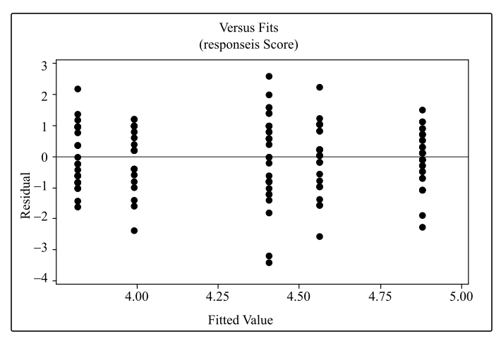
Interpretation: From the above graph, it is observed that the scatter plot of the residuals is symmetrically scattered below and above the zero and there are two outliers below the zero but these are not the extreme outliers.

(b)

To determine

Whether the spread of the residual of each group is relatively equal or not.

Answer to Problem 22E

Solution: Yes, the spread of the residual of each group is relatively equal.

Explanation of Solution

From the scatterplot of the residuals versus the group variables in part (a), it is observed that the residuals are symmetrically scattered below and above the zero. It implies that the spread of the residual of each group is relatively equal.

(c)

To determine

To graph: The Normal quantile plot of the residuals obtained in part (a) and identify whether it is normal or not.

Explanation of Solution

Graph:

Use Minitab to graph the Normal quantile plot as below:

Step1: Enter the provided data in the worksheet.

Step2: Select stat> ANOVA>one-way analysis of variance.

Step3: Select Score in the Response and Friends in the Factor.

Step4: Click on Graphs and select the Normal plot of residuals and then press OK.

Step5: Press OK.

The obtained graph is,

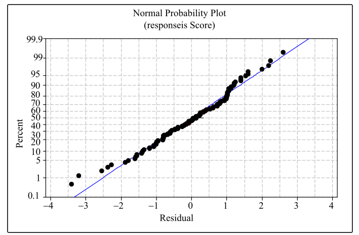
Interpretation: From the obtained graph, it is observed that the normal quantile plot is nearly fitted to the line. Hence, the residual is approximately normal.