
Concept explainers
Videos
a.
Perform a hypothesis test to determine if the population proportion of good parts is the same for all three shifts at
Find the p-value and draw conclusion.
a.
Answer to Problem 27SE
All population proportions for three shifts are not equal.
The p-value is 0.0174.
Explanation of Solution
Calculation:
The given data related to the quality (good and defective) of goods for first, second and third shifts.
Let
State the test hypotheses:
Null hypothesis:
That is, all population proportions for three shifts are equal.
Alternative hypothesis:
That is, not all population proportions for three shifts are equal.
The row and column total is tabulated below:
| Quality | First Shift | Second Shift | Third Shift | Total |
| Good | 285 | 368 | 176 | 829 |
| Defective | 15 | 32 | 24 | 71 |
| Total | 300 | 400 | 200 | 900 |
The formula for expected frequency is given below:
The expected frequency for each category is calculated as follows:
| Quality | First Shift | Second Shift | Third Shift |
| Good | |||
| Defective |
The formula for chi-square test statistic is given as,
Therefore, the value of chi-square test statistic is,
Thus, the chi-square test statistic is 8.10.
Degrees of freedom:
Thus, the degree of freedom is 2.
Level of significance:
The given level of significance is
p-value:
Software procedure:
Step -by-step software procedure to obtain p-value using MINITAB software is as follows:
- Select Graph > Probability distribution plot > view probability
- Select chi-square under distribution and enter 2 in degrees of freedom.
- Enter the X-value as 8.10 under shaded area.
- Select OK.
- Output using MINITAB software is given below:
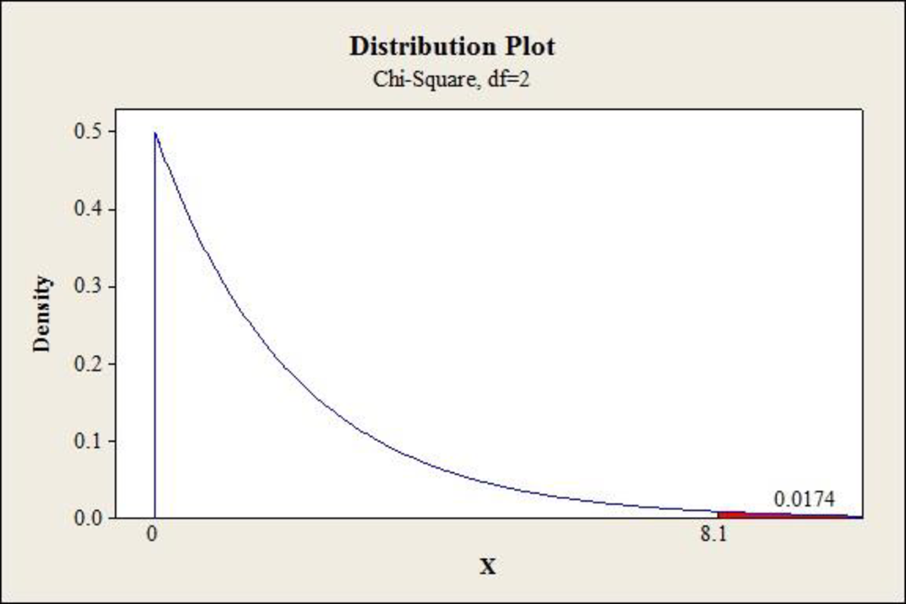
From the MINITAB output, the p-value is 0.0174.
Rejection rule:
If the
Conclusion:
Here, the p-value less than the level of significance.
That is,
Thus, the decision is “reject the null hypothesis”.
Therefore, the data provide sufficient evidence to conclude that not all population proportions for three shifts are equal. That is, the shifts differ in terms of production quality.
b.
Perform a multiple comparison test to determine how the shifts differ in terms of quality.
b.
Answer to Problem 27SE
Supplier A and B can be used as they are not significantly different in terms of the proportion defective components and supplier C can be eliminated due to higher proportion of defective components.
Explanation of Solution
Calculation:
The critical values for pairwise comparison procedure of k population proportions are given as,
Where,
The sample proportion of good item for first shift is,
The sample proportion of good item for second shift is,
The sample proportion of good item for third shift is,
Multiple comparisons for first and second shift:
Degrees of freedom:
For a population of size k, the degrees of freedom is given as
In this given problem, for three populations the degrees of freedom is,
Thus, the degree of freedom is 2.
Level of significance:
The given level of significance is
From the table “Area in Upper Tail” table it is found that the highest
Thus, the critical values for pairwise comparison procedure of first and second shift is,
Multiple comparisons for first and third shift:
Degrees of freedom:
For a population of size k, the degrees of freedom is given as
In this given problem, for three populations the degrees of freedom is
Level of significance:
The given level of significance is
From the table “Area in Upper Tail” table it is found that the highest
Thus, the critical values for pairwise comparison procedure of first and third shift is,
Multiple comparisons for second and third shift:
Degrees of freedom:
For a population of size k, the degrees of freedom is given as
In this given problem, for three populations the degrees of freedom is
Level of significance:
The given level of significance is
From the table “Area in Upper Tail” table it is found that the highest
Thus, the critical values for pairwise comparison procedure of supplier B and C is,
Now,
| Comparison |
Difference |
Critical Value |
Significant | ||||
| First vs. second | 0.95 | 0.92 | 0.03 | 300 | 400 | 0.0453 | No |
| First vs. Third | 0.95 | 0.88 | 0.07 | 300 | 200 | 0.0641 | Yes |
| Second vs. Third | 0.92 | 0.88 | 0.04 | 400 | 200 | 0.0653 | No |
Conclusion:
It can be concluded that first and third shift, both are significantly different from second shift. Due to proportion of defective goods than other shifts, third shift can be eliminated.
Thus, the shift first and third can be used as they are not significantly different in terms of the proportion good components.
Want to see more full solutions like this?
Chapter 12 Solutions
MindTap Business Statistics, 1 term (6 months) Printed Access Card for Anderson/Sweeney/Williams/Camm/Cochran's Essentials of Statistics for Business and Economics, 8th


 Glencoe Algebra 1, Student Edition, 9780079039897...AlgebraISBN:9780079039897Author:CarterPublisher:McGraw Hill
 College Algebra (MindTap Course List)AlgebraISBN:9781305652231Author:R. David Gustafson, Jeff HughesPublisher:Cengage Learning