
Concept explainers
Videos
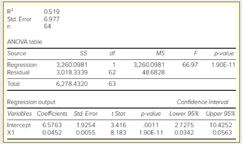
In the following regression, X = total assets ($ billions), Y = total revenue ($ billions), and n = 64 large banks. (a) Write the fitted regression equation. (b) State the degrees of freedom for a two-tailed test for zero slope, and use Appendix D to find the critical value at α = .05. (c) What is your conclusion about the slope? (d) Interpret the 95 percent confidence limits for the slope. (e) Verify that F= t2 for the slope. (f) In your own words, describe the fit of this regression.
a.
Write the fitted regression equation.
Answer to Problem 62CE
The regression equation is,
Explanation of Solution
Calculation:
An output of a regression is given. The X variable is the total assets and Y be the total revenue.
Regression:
Suppose
Where,
The total sum of squares is denoted as,
The regression sum of squares is denoted as,
The error sum of squares is denoted as,
From the regression the fitted line is denoted as,
From the output,
Hence, the regression equation is,
b.
Find the degrees of freedom for the two-tailed test for zero slope.
Find the critical value at 0.05 level of significanceusing Appendix D.
Answer to Problem 62CE
The degrees of freedom for the two-tailed test for zero slop is62.
The critical value at 0.05 level of significanceis 2.000.
Explanation of Solution
Calculation:
Critical value:
Here from the output, the sample size,
The degrees of freedom is,
For two tailed test, the critical value for t-test will be,
From the Appendix D: STUDENT’S t CRITICAL VALUES:
- • Since 62 is not in the table, so locate the value 60in the column of degrees of freedom.
- • Locate the 0.025 in level of significance.
- • The intersecting value that corresponds to the degrees of freedom 60 with level of significance 0.025 is 2.000.
Thus, the critical-valueusing Appendix D is 2.000.
c.
Make a conclusion about the slope.
Explanation of Solution
Let
Hypotheses:
Null hypothesis:
That is, the slope is zero.
Alternative hypothesis:
That is, the slope is not equal to zero.
Decision rule:
If
If
From the output, the t-statistics is 8.183 and from part (b), the critical value at 0.05 level of significanceis 2.000.
Conclusion:
Here the t-statistics is greater than the critical value at 0.05 level of significance.
That is,
Hence, by the decision rule reject the null hypothesis.
That is, the slope is significantly different from zero.
d.
Interpret the 95% confidence interval for the slope.
Explanation of Solution
The 95% confidence interval for the slope,
Where,
From the output, the 95% confidence interval of the slope is (0.0342, 0.0563).
Interpretation:
From the confidence interval it can be concluded that there is 95% confident that the slope will lie between 0.0342 and 0.0563.
e.
Verify
Explanation of Solution
Calculation:
From the output the F statistic is 66.97.
For the slope the t-statistic is 8.183.
Hence, it can be concluded that
f.
Describe the fit of the regression.
Explanation of Solution
Calculation:
From the output, the R-squared value is 0.519.
The coefficient of determination (
The
Want to see more full solutions like this?
Chapter 12 Solutions
Applied Statistics in Business and Economics


- Find the equation of the regression line for the following data set. x 1 2 3 y 0 3 4arrow_forwardFor the following exercises, use Table 4 which shows the percent of unemployed persons 25 years or older who are college graduates in a particular city, by year. Based on the set of data given in Table 5, calculate the regression line using a calculator or other technology tool, and determine the correlation coefficient. Round to three decimal places of accuracyarrow_forwardFor a linear regression for a sample of n=20 pairs of X and Y values. What is the value of the degrees of freedom for the predicted portion of the Y-score variance, MSregression?arrow_forward
- A sociologist was hired by a large city hospital to investigate the relationship between the number of unauthorized days that employees are absent per year and the distance (miles) between home and work for the employee. A sample of 10 employees was chosen, and the following data were collected. A. Is the estimated regression equation appropriate and adequatearrow_forwardGiven a generic data set (x,y) with a linear regression. How do you determine if the y(dependent) will be less than a certain value?arrow_forwardSuppose the following data were collected from a sample of 15 houses relating selling price to square footage and the architectural style of the house. Use statistical software to find the following regression equation: PRICEi=b0+b1SQFTi+b2COLONIALi+b3RANCHi+ei . Is there enough evidence to support the claim that on average, houses that are ranch style have lower selling prices than houses that are Victorian style at the 0.05 level of significance? If yes, write the regression equation in the spaces provided with answers rounded to two decimal places. Else, select "There is not enough evidence."Selling Price Square Footage Colonial (1 if house is Colonial style, 0 otherwise) Ranch (1 if house is Ranch style, 0 otherwise) Victorian (1 if house is Victorian style, 0 otherwise) 377640 1941 1 0 0 460996 3397 0 1 0 405781 2764 0 0 1 407216 2906 0 0 1 435139 3401 1 0 0 405275 2600 0 0 1 381141 2203 0 1 0 370490 2046 1 0 0 404070 2210 0 0 1 460196 3692 0 1 0 382780 2172 1 0 0 406466 2606 0 1…arrow_forward
- In a linear regression, if you do not sample all across the x variables in a study and are only having values in the middle of your graph and none at the low and high values for x, what type of error could you mistakenly carry out?arrow_forwardIn a regression context, under what situation is the predicted value for Y equal to the mean of Y?arrow_forwarda. Can you construct a 95% confidence interval for the y intercept for the regression equation then justify the correlation between time and duration? b. Also, what are the chances of seeing a relationship between time and duration as strong or stronger than this, when in fact there was none?arrow_forward
- In simple linear regression, most often we perform a two-tail test of the population slope 1 to determine whether there is sufficient evidence to infer that a linear relationship exists. The null hypothesis is stated as:arrow_forwardIf a new independent variable is added to a regression equation, the adjusted R2 increases only if the absolute value of the t-statistic of the new variable is greater than one. Group of answer choices True False.arrow_forwardon the basis of the value of linear correlation coefficient, would you conclude, at the /r/>0.9 level, that the data can be reasonably modeled linear equation?arrow_forward

 Glencoe Algebra 1, Student Edition, 9780079039897...AlgebraISBN:9780079039897Author:CarterPublisher:McGraw Hill
 Functions and Change: A Modeling Approach to Coll...AlgebraISBN:9781337111348Author:Bruce Crauder, Benny Evans, Alan NoellPublisher:Cengage Learning