
Concept explainers
Videos
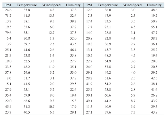
Air pollution: Following are measurements of particulate matter (PM) concentration (in micrograms per cubic meter), temperature, in degrees Fahrenheit wind speed in miles per hour, and humidity in percent for 38 days in Denver, Colorado.
- Let y represent PM,
- Predict the particulate concentration on a day where the temperature is 40 degrees, the wind speed is 5 miles per hour, and the humidity is 30 percent.
- Refer to part (b). Construct a 95% confidence interval for the particulate concentration.
- Refer to part (b). Construct a 95% prediction interval for the particulate concentration.
- Are all the values in the prediction interval reasonable? Explain.
- What percentage of the variation in particulate concentration is explained by the model?
- Is the model useful for prediction? Why or why not? Use the
- Test
(a)
The multiple regression equation
Answer to Problem 11RE
Explanation of Solution
It is known that for estimating coefficient below given formula is used
Where,
Now, using ‘R’ software coefficients are calculated.
(b)
The particulate concentration on a day where temperature, wind speed and humidity is
Answer to Problem 11RE
Explanation of Solution
From part (a)
Now putting the values of
Using calculator,
(c)
The 95% confidence interval for the particulate concentration
Answer to Problem 11RE
The 95% confidence interval for the particulate concentration is given below:
| fitted | lower | upper |
| 20.47848 | 15.11886 | 25.8381 |
| 52.31326 | 41.71678 | 62.90975 |
| 40.00498 | 32.93215 | 47.07781 |
| 24.39183 | 18.80337 | 29.98028 |
| 48.76496 | 38.10801 | 59.42191 |
| 12.63185 | 4.863304 | 20.40039 |
| 17.92577 | 12.6039 | 23.24764 |
| 23.18885 | 16.01585 | 30.36184 |
| 17.51326 | 10.06084 | 24.96568 |
| 20.19053 | 14.54028 | 25.84077 |
| 53.03338 | 43.31002 | 62.75673 |
| 19.38092 | 11.9622 | 26.79964 |
| 11.56664 | 3.850621 | 19.28265 |
| 9.147208 | 1.815757 | 16.47866 |
| 25.77363 | 19.68499 | 31.86227 |
| 37.31334 | 29.49157 | 45.13512 |
| 41.46232 | 32.1341 | 50.79054 |
| 40.68683 | 31.59058 | 49.78308 |
| 25.38821 | 19.62186 | 31.15456 |
| 20.29095 | 14.17048 | 26.41141 |
| 9.484433 | 0.412967 | 18.5559 |
| 21.81731 | 15.19766 | 28.43697 |
| 22.40822 | 13.90819 | 30.90825 |
| 15.21627 | 7.948146 | 22.48438 |
| 17.56946 | 11.07772 | 24.0612 |
| 12.52526 | 6.282131 | 18.76839 |
| 14.68255 | 7.538868 | 21.82623 |
| 16.894 | 8.889021 | 24.89897 |
| 18.27573 | 10.99998 | 25.55148 |
| 17.17309 | 9.305811 | 25.04037 |
| 27.14994 | 21.18848 | 33.11141 |
| 25.14871 | 16.67252 | 33.62489 |
| 24.66506 | 16.59167 | 32.73845 |
| 27.16704 | 18.07744 | 36.25665 |
| 33.64924 | 25.76426 | 41.53423 |
| 43.80541 | 35.69192 | 51.9189 |
| 21.51525 | 17.32562 | 25.70487 |
| 35.60585 | 29.60614 | 41.60555 |
Explanation of Solution
It is known that,
Confidence interval for dependent variable is given by
Where,
Using ‘R’ programming 95% confidence interval has been calculated.
| fitted | lower | upper |
| 20.47848 | 15.11886 | 25.8381 |
| 52.31326 | 41.71678 | 62.90975 |
| 40.00498 | 32.93215 | 47.07781 |
| 24.39183 | 18.80337 | 29.98028 |
| 48.76496 | 38.10801 | 59.42191 |
| 12.63185 | 4.863304 | 20.40039 |
| 17.92577 | 12.6039 | 23.24764 |
| 23.18885 | 16.01585 | 30.36184 |
| 17.51326 | 10.06084 | 24.96568 |
| 20.19053 | 14.54028 | 25.84077 |
| 53.03338 | 43.31002 | 62.75673 |
| 19.38092 | 11.9622 | 26.79964 |
| 11.56664 | 3.850621 | 19.28265 |
| 9.147208 | 1.815757 | 16.47866 |
| 25.77363 | 19.68499 | 31.86227 |
| 37.31334 | 29.49157 | 45.13512 |
| 41.46232 | 32.1341 | 50.79054 |
| 40.68683 | 31.59058 | 49.78308 |
| 25.38821 | 19.62186 | 31.15456 |
| 20.29095 | 14.17048 | 26.41141 |
| 9.484433 | 0.412967 | 18.5559 |
| 21.81731 | 15.19766 | 28.43697 |
| 22.40822 | 13.90819 | 30.90825 |
| 15.21627 | 7.948146 | 22.48438 |
| 17.56946 | 11.07772 | 24.0612 |
| 12.52526 | 6.282131 | 18.76839 |
| 14.68255 | 7.538868 | 21.82623 |
| 16.894 | 8.889021 | 24.89897 |
| 18.27573 | 10.99998 | 25.55148 |
| 17.17309 | 9.305811 | 25.04037 |
| 27.14994 | 21.18848 | 33.11141 |
| 25.14871 | 16.67252 | 33.62489 |
| 24.66506 | 16.59167 | 32.73845 |
| 27.16704 | 18.07744 | 36.25665 |
| 33.64924 | 25.76426 | 41.53423 |
| 43.80541 | 35.69192 | 51.9189 |
| 21.51525 | 17.32562 | 25.70487 |
| 35.60585 | 29.60614 | 41.60555 |
(d)
The 95% prediction interval for the particulate concentration
Answer to Problem 11RE
The 95% prediction interval for the particulate concentration is given below
| fitted | lower | upper |
| 20.47848 | -3.39044 | 44.3474 |
| 52.31326 | 26.75382 | 77.87271 |
| 40.00498 | 15.69398 | 64.31598 |
| 24.39183 | 0.470482 | 48.31317 |
| 48.76496 | 23.18039 | 74.34954 |
| 12.63185 | -11.8906 | 37.15429 |
| 17.92577 | -5.9347 | 41.78625 |
| 23.18885 | -1.15149 | 47.52918 |
| 17.51326 | -6.91088 | 41.93739 |
| 20.19053 | -3.74533 | 44.12638 |
| 53.03338 | 27.82339 | 78.24336 |
| 19.38092 | -5.03296 | 43.79479 |
| 11.56664 | -12.9392 | 36.07249 |
| 9.147208 | -15.2403 | 33.53471 |
| 25.77363 | 1.730515 | 49.81675 |
| 37.31334 | 12.77398 | 61.8527 |
| 41.46232 | 16.40208 | 66.52256 |
| 40.68683 | 15.71201 | 65.66165 |
| 25.38821 | 1.424684 | 49.35174 |
| 20.29095 | -3.76025 | 44.34214 |
| 9.484433 | -15.4814 | 34.45024 |
| 21.81731 | -2.36573 | 46.00036 |
| 22.40822 | -2.35567 | 47.17211 |
| 15.21627 | -9.15227 | 39.5848 |
| 17.56946 | -6.57888 | 41.7178 |
| 12.52526 | -11.5574 | 36.60796 |
| 14.68255 | -9.64916 | 39.01425 |
| 16.894 | -7.70437 | 41.49236 |
| 18.27573 | -6.09508 | 42.64654 |
| 17.17309 | -7.38081 | 41.72699 |
| 27.14994 | 3.13872 | 51.16117 |
| 25.14871 | 0.392989 | 49.90442 |
| 24.66506 | 0.044349 | 49.28577 |
| 27.16704 | 2.194643 | 52.13945 |
| 33.64924 | 9.089665 | 58.20882 |
| 43.80541 | 19.17152 | 68.4393 |
| 21.51525 | -2.11848 | 45.14897 |
| 35.60585 | 11.5851 | 59.62659 |
Explanation of Solution
It is known that,
Prediction interval for dependent variable is given by
Where,
Using ‘R’ programming 95% prediction interval has been calculated.
| fitted | lower | upper |
| 20.47848 | -3.39044 | 44.3474 |
| 52.31326 | 26.75382 | 77.87271 |
| 40.00498 | 15.69398 | 64.31598 |
| 24.39183 | 0.470482 | 48.31317 |
| 48.76496 | 23.18039 | 74.34954 |
| 12.63185 | -11.8906 | 37.15429 |
| 17.92577 | -5.9347 | 41.78625 |
| 23.18885 | -1.15149 | 47.52918 |
| 17.51326 | -6.91088 | 41.93739 |
| 20.19053 | -3.74533 | 44.12638 |
| 53.03338 | 27.82339 | 78.24336 |
| 19.38092 | -5.03296 | 43.79479 |
| 11.56664 | -12.9392 | 36.07249 |
| 9.147208 | -15.2403 | 33.53471 |
| 25.77363 | 1.730515 | 49.81675 |
| 37.31334 | 12.77398 | 61.8527 |
| 41.46232 | 16.40208 | 66.52256 |
| 40.68683 | 15.71201 | 65.66165 |
| 25.38821 | 1.424684 | 49.35174 |
| 20.29095 | -3.76025 | 44.34214 |
| 9.484433 | -15.4814 | 34.45024 |
| 21.81731 | -2.36573 | 46.00036 |
| 22.40822 | -2.35567 | 47.17211 |
| 15.21627 | -9.15227 | 39.5848 |
| 17.56946 | -6.57888 | 41.7178 |
| 12.52526 | -11.5574 | 36.60796 |
| 14.68255 | -9.64916 | 39.01425 |
| 16.894 | -7.70437 | 41.49236 |
| 18.27573 | -6.09508 | 42.64654 |
| 17.17309 | -7.38081 | 41.72699 |
| 27.14994 | 3.13872 | 51.16117 |
| 25.14871 | 0.392989 | 49.90442 |
| 24.66506 | 0.044349 | 49.28577 |
| 27.16704 | 2.194643 | 52.13945 |
| 33.64924 | 9.089665 | 58.20882 |
| 43.80541 | 19.17152 | 68.4393 |
| 21.51525 | -2.11848 | 45.14897 |
| 35.60585 | 11.5851 | 59.62659 |
(e)
The percentage of variation in particulate concentrationas explained by the model.
Answer to Problem 11RE
The percentage of variation in particulate concentrationas explained by the model is
Explanation of Solution
It is known that,
R-squared (R2) is a statistical measure that represents the proportion of the variance for a dependent variable that's explained by an independent variable or variables in a regression model.
In case of multiple regression, adjusted R-squared is used.
Using ‘R’ programming adjusted R-squared is calculated.
The percentage of variation in particulate concentration as explained by the model is
(f)
Whether the model is useful for prediction or not.
Explanation of Solution
While fitting the model many regression assumptions like autocorrelation, multi-collinearity, heteroscedasticity etc. have not been checked.
So, one cannot say anything about the efficiency and accuracy. One has to consider some other measure like AIC, BIC etc. apart from
(g)
Whether one can reject
Answer to Problem 11RE
| Coefficients | P-value. |
At
Explanation of Solution
Let’s declare null hypothesis,
It is known that for this test, test-statistic is given by
Where,
RSS is residual sum of square
Using ‘R’ software p-values for the test is calculated.
| Coefficients | P-value. |
At
‘R’ code:
PM=c(24.6,71.7,13.7,19.5,79.6,6.4,13.9,25.1,21.3,19.0,33.5,37.8,8.0,15.1,27.9,35.4,22.0,45.4,23.7
     ,12.6,7.3,17.4,7.7,14.0,20.8,19.8,13.1,10.5,22.7,24.0,39.1,28.2,41.9,25.7,30.1,49.1,11.5,27.1)
Temperature=c(35.8,41.5,38.1,35.6,35.1,30.8,39.7,44.6,53.8,52.5,48.2,29.6,31.7,41.5,55.1,59.9,62.6,51.3,41.5
              ,36.0,47.9,33.5,25.1,28.5,32.8,36.9,43.7,48.3,54.9,57.8,49.2,51.6,54.2,53.8,60.6,44.2,40.9,39.6)
Wind_Speed=c(4.8,13.3,9.5,6.0,12.7,1.3,2.5,2.6,1.4,3.3,11.9,3.2,3.1,2.0,5.2,8.0,9.3,10.7,6.5
             ,3.0,2.5,3.5,4.5,3.1,4.4,2.7,3.8,4.5,3.6,2.7,4.0,2.5,2.6,2.8,5.7,8.7,3.9,7.3)
Humidity=c(37.8,32.6,39.2,37.2,37.5,52.0,43.5,46.4,33.8,27.9,35.1,53.0,37.8,29.5,22.6,19.4,15.3,17.9,29.1,48.6
           ,19.7,50.9,55.1,47.7,38.7,36.1,25.2,19.4,20.0,20.5,39.2,42.5,38.1,41.6,26.8,43.9,39.5,43.8)


# (a)
linear.model=lm(PM~Temperature+Wind_Speed+Humidity)
summ=summary(linear.model)
summ$coefficients
##                Estimate Std. Error   t value     Pr(>|t|)
## (Intercept) -42.5163427 20.9064691 -2.033645 4.985097e-02
## Temperature   0.6557601  0.2791580  2.349065 2.477066e-02
## Wind_Speed    3.6607217  0.6053612  6.047170 7.480612e-07
## Humidity      0.5806123  0.2598741  2.234206 3.215189e-02
#(b)
y=-42.5163427+(0.6557601)*40+( 3.6607217)*5+(0.5806123)*30
y
## [1] 19.43604
#(c)
predict(linear.model, interval ='confidence')
##          fit        lwrupr
## 1  20.478479 15.1188573 25.83810
## 2  52.313262 41.7167782 62.90975
## 3  40.004976 32.9321466 47.07781
## 4  24.391825 18.8033699 29.98028
## 5  48.764964 38.1080145 59.42191
## 6  12.631847  4.8633035 20.40039
## 7  17.925773 12.6039026 23.24764
## 8  23.188846 16.0158506 30.36184
## 9  17.513258 10.0608350 24.96568
## 10 20.190528 14.5402823 25.84077
## 11 53.033375 43.3100223 62.75673
## 12 19.380918 11.9621970 26.79964
## 13 11.566635  3.8506207 19.28265
## 14  9.147208  1.8157572 16.47866
## 15 25.773630 19.6849908 31.86227
## 16 37.313340 29.4915657 45.13512
## 17 41.462320 32.1341000 50.79054
## 18 40.686834 31.5905824 49.78308
## 19 25.388211 19.6218624 31.15456
## 20 20.290945 14.1704778 26.41141
## 21  9.484433  0.4129668 18.55590
## 22 21.817313 15.1976555 28.43697
## 23 22.408222 13.9081921 30.90825
## 24 15.216265  7.9481455 22.48438
## 25 17.569461 11.0777219 24.06120
## 26 12.525258  6.2821313 18.76839
## 27 14.682547  7.5388682 21.82623
## 28 16.893997  8.8890210 24.89897
## 29 18.275732 10.9999846 25.55148
## 30 17.173093  9.3058109 25.04037
## 31 27.149944 21.1884829 33.11141
## 32 25.148706 16.6725233 33.62489
## 33 24.665061 16.5916728 32.73845
## 34 27.167044 18.0774358 36.25665
## 35 33.649244 25.7642561 41.53423
## 36 43.805413 35.6919222 51.91890
## 37 21.515247 17.3256230 25.70487
## 38 35.605845 29.6061374 41.60555
#(d)
predict(linear.model, interval ='prediction')
## Warning in predict.lm(linear.model, interval = "prediction"): predictions on current data refer to _future_ responses
##          fit          lwrupr
## 1  20.478479  -3.39044242 44.34740
## 2  52.313262  26.75381513 77.87271
## 3  40.004976  15.69397519 64.31598
## 4  24.391825   0.47048157 48.31317
## 5  48.764964  23.18039033 74.34954
## 6  12.631847 -11.89059426 37.15429
## 7  17.925773  -5.93469948 41.78625
## 8  23.188846  -1.15148528 47.52918
## 9  17.513258  -6.91087916 41.93739
## 10 20.190528  -3.74532639 44.12638
## 11 53.033375  27.82338810 78.24336
## 12 19.380918  -5.03295643 43.79479
## 13 11.566635 -12.93921571 36.07249
## 14  9.147208 -15.24028905 33.53471
## 15 25.773630   1.73051529 49.81675
## 16 37.313340  12.77398400 61.85270
## 17 41.462320  16.40208203 66.52256
## 18 40.686834  15.71201353 65.66165
## 19 25.388211   1.42468407 49.35174
## 20 20.290945  -3.76025018 44.34214
## 21  9.484433 -15.48137046 34.45024
## 22 21.817313  -2.36573281 46.00036
## 23 22.408222  -2.35567035 47.17211
## 24 15.216265  -9.15226841 39.58480
## 25 17.569461  -6.57888343 41.71780
## 26 12.525258 -11.55744274 36.60796
## 27 14.682547  -9.64916086 39.01425
## 28 16.893997  -7.70436657 41.49236
## 29 18.275732  -6.09507770 42.64654
## 30 17.173093  -7.38080679 41.72699
## 31 27.149944   3.13872014 51.16117
## 32 25.148706   0.39298914 49.90442
## 33 24.665061   0.04434892 49.28577
## 34 27.167044   2.19464261 52.13945
## 35 33.649244   9.08966541 58.20882
## 36 43.805413  19.17152225 68.43930
## 37 21.515247  -2.11847504 45.14897
## 38 35.605845  11.58509698 59.62659
#(e)
summ$adj.r.squared
## [1] 0.4969786
# (f), (g)
summ$coefficients
##                Estimate Std. Error   t value     Pr(>|t|)
## (Intercept) -42.5163427 20.9064691 -2.033645 4.985097e-02
## Temperature   0.6557601  0.2791580  2.349065 2.477066e-02
## Wind_Speed    3.6607217  0.6053612  6.047170 7.480612e-07
## Humidity      0.5806123  0.2598741  2.234206 3.215189e-02
Want to see more full solutions like this?
Chapter 13 Solutions
Elementary Statistics ( 3rd International Edition ) Isbn:9781260092561


- If your graphing calculator is capable of computing a least-squares sinusoidal regression model, use it to find a second model for the data. Graph this new equation along with your first model. How do they compare?arrow_forwardOlympic Pole Vault The graph in Figure 7 indicates that in recent years the winning Olympic men’s pole vault height has fallen below the value predicted by the regression line in Example 2. This might have occurred because when the pole vault was a new event there was much room for improvement in vaulters’ performances, whereas now even the best training can produce only incremental advances. Let’s see whether concentrating on more recent results gives a better predictor of future records. (a) Use the data in Table 2 (page 176) to complete the table of winning pole vault heights shown in the margin. (Note that we are using x=0 to correspond to the year 1972, where this restricted data set begins.) (b) Find the regression line for the data in part ‚(a). (c) Plot the data and the regression line on the same axes. Does the regression line seem to provide a good model for the data? (d) What does the regression line predict as the winning pole vault height for the 2012 Olympics? Compare this predicted value to the actual 2012 winning height of 5.97 m, as described on page 177. Has this new regression line provided a better prediction than the line in Example 2?arrow_forwardThe electric power consumed each month by a chemical plant is thought to be related to the average ambient temperature (x1), the number of days in the month (x2). The past year’s historical data are available and are presented in the following table: Fit a multiple linear regression model to these data.arrow_forward
- A negative correlation between variables X and Y will always result in a positive slope in the linear regression model. Cannot tell from the given information. False Truearrow_forwardCan a causal relationship be established between a variable y and a variable x by running the following regressions: i) y = f(x) and ii) x = f(y). Explain in less than 75 words.arrow_forwardFour pairs of data yield r= 0.942 and regression equation y=3x.Also, y= 12.75. What is the best predicted value of y for x= 2.9?arrow_forward
- What is the equation for a simple linear regression model with one independent variable (x) and one dependent variable (y)?arrow_forward1. How would you go about setting up using this Linear Regression model applying both of the Y & X model. What represents the Y and what represents the X variables? 2. Would you suppose the Y = Bo + B1X + E equations to have a negative or positive slope in this example. 3. What would be the grade results if you decided to watch NETFLIX videos instead? What would that slope look like. 4. How would you go about getting the needed X and Y linear regression samples to create a study like the Grade vs. Time study example? What is one X, Y example you could imagine applying in your own life? Without doing this assignment use what you are learning about 5. Dallas Cowboy Stadium Forecasting Question. I added a problem that is going to make you think and that is what Q 5 is to get you to do. The Dallas Cowboys want to know how many more people they are expecting to come to their future games. Their building is alright maxed out but they need to know about the growth of ticket sales to…arrow_forwardIn a fisheries researcher's experiment, the correlation between the number of eggs in the nest and the number of viable (surviving) eggs for a sample of nests is r = 0.67. The equation of the regression line for number of viable eggs y versus number of eggs in the nest x is y = 0.72x + 17.07. For a nest with 140 eggs, what is the predicted number of viable eggs?arrow_forward
- Why do we have in general, two lines of regression? Obtain the regression of Y on X and X on Y from the following table and estimate the blood pressure when the age is 45. Also give the interpretation.arrow_forwardA group of scientists and engineers aim to create fuel-efficient and fuel-efficient cars. In order to study the problem, they randomly selected a sample of 20 cars and took information from X: weight (hundreds of pounds) and Y: vehicle performance (mill / gal). Once the information was collected and analyzed, using a scatterplot, they determined that a linear model can fit the data. Using R the following information is obtained from the linear regression model. Y = 40.15−0.513X According to the model, what would be the weight of a car with a performance of 14 mill / gal? Select one: a. -39.98 lbs b. 39.98 lb c. 77.82 lb d. -77.82 lbarrow_forward
 Algebra & Trigonometry with Analytic GeometryAlgebraISBN:9781133382119Author:SwokowskiPublisher:Cengage
 College AlgebraAlgebraISBN:9781305115545Author:James Stewart, Lothar Redlin, Saleem WatsonPublisher:Cengage Learning
 Trigonometry (MindTap Course List)TrigonometryISBN:9781305652224Author:Charles P. McKeague, Mark D. TurnerPublisher:Cengage Learning
 Algebra and Trigonometry (MindTap Course List)AlgebraISBN:9781305071742Author:James Stewart, Lothar Redlin, Saleem WatsonPublisher:Cengage Learning