Chapter 13, Problem 12RE

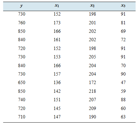
Icy lakes: Following are data on maximum ice thickness in millimeters (y): average number of days per year of ice cover $(x_1)$, average number of days the bottom temperature is lower than 8°C $(x_2)$. and the average snow depth in millimeters $(x_3)$ for 13 lakes in Minnesota

1. Construct the multiple regression equation $\hat{y}=b_0+b_1{x}_1+b_2{x}_2+b_3{x}_3$.
2. Predict the ice thickness for a lake which is covered by ice an average of 140 days per year, the bottom temperature is less than 8°C an average of 190 days per year, and the average snow depth is 60 millimeters.
3. Refer to part (b). Construct a 95% confidence interval for the ice thickness.
4. Refer to part (b). Construct a 95?-’o prediction interval for the ice thickness.
5. What percentage of the variation in ice thickness is explained by the model?
6. Is the model useful for prediction? Why or why not? Use the $\alpha =0.05$ level.
7. Test $H_0:{\beta }_1=0$ versus $H_1:{\beta }_1\ne 0$ at the $\alpha =0.05$ level. Can you reject $H_0$ ? Repeat for ${\beta }_2$ and ${\beta }_3$.

To determine

The multiple regression equation $\hat{y}=b_0+b_1{x}_1+b_2{x}_2+b_3{x}_3$

Answer to Problem 12RE

  $\hat{y}=-356.867508+(3.518179)x_1+(3.679930)x_2+(-2.187464)x_3$

Explanation of Solution

It is known that for estimating coefficient below given formula is used

  $b = {\left(X\text{'}X\right)}^{-1}X\text{'}Y$

Where,

  $b=\left[\begin{array}{l}{b}_0\\ b_1\\ b_2\\ b_3\end{array}\right]$ And $X$ is the matrix of observations.

Now, using ‘R’ software coefficients are calculated.

  $\begin{array}{l}\hat{y}=b_0+b_1{x}_1+b_2{x}_2+b_3{x}_3\\ \hat{y}=-356.867508+(3.518179)x_1+(3.679930)x_2+(-2.187464)x_3\end{array}$

To determine

The ice thickness for a lake who’s set of values are $(140,190,60)$ .

Answer to Problem 12RE

  $\hat{y}=703.6164$

Explanation of Solution

From part (a)

  $\hat{y}=-356.867508+(3.518179)x_1+(3.679930)x_2+(-2.187464)x_3$

Now putting the values of $(x_1,x_2,x_3)$ as $(140,190,60)$ in the above equation.

Using calculator,

  $\hat{y}=703.6164$

To determine

The 95% confidence interval for the ice thickness

Answer to Problem 12RE

The 95% confidence interval for the ice thickness is given below

fitted	lower	upper
707.4625	664.5821	750.343
814.2587	760.425	868.0925
819.561	774.5556	864.5664
795.4077	762.989	827.8264
707.4625	664.5821	750.343
736.7402	696.8865	776.594
824.7334	780.4485	869.0182
749.3205	713.7654	784.8755
651.7419	573.7127	729.7712
815.8782	747.2412	884.5152
743.6261	704.3767	782.8756
791.1259	743.0253	839.2265
721.6812	684.1523	759.2101

Explanation of Solution

It is known that,

Confidence interval for dependent variable is given by

  ${\hat{y}}_h\pm t_{\frac{\alpha }{2},n-2}\sqrt{MSE\left(\frac{1}{n}+\frac{{\left(x_k-\stackrel{\_}{x}\right)}^2}{{\displaystyle \sum _{i=1}^n\left(X_i-\stackrel{\_}{x^2}\right)}}\right)}$

Where,

  ${\hat{y}}_h$ is the fitted response variable

  $\sqrt{MSE\left(\frac{1}{n}+\frac{{\left(x_k-\stackrel{\_}{x}\right)}^2}{{\displaystyle \sum _{i=1}^n\left(X_i-\stackrel{\_}{x^2}\right)}}\right)}$ is the standard error of the fit

Using ‘R’ programming 95% confidence interval has been calculated.

fitted	lower	upper
707.4625	664.5821	750.343
814.2587	760.425	868.0925
819.561	774.5556	864.5664
795.4077	762.989	827.8264
707.4625	664.5821	750.343
736.7402	696.8865	776.594
824.7334	780.4485	869.0182
749.3205	713.7654	784.8755
651.7419	573.7127	729.7712
815.8782	747.2412	884.5152
743.6261	704.3767	782.8756
791.1259	743.0253	839.2265
721.6812	684.1523	759.2101

To determine

The 95% prediction interval for the ice thickness

Answer to Problem 12RE

The 95% prediction interval for the ice thickness is given below

fitted	lower	upper
707.4625	610.1451	804.78
814.2587	711.6428	916.8747
819.561	721.2887	917.8333
795.4077	702.2255	888.5899
707.4625	610.1451	804.78
736.7402	640.7179	832.7625
824.7334	726.789	922.6778
749.3205	655.0012	843.6397
651.7419	534.6073	768.8766
815.8782	704.7792	926.9772
743.6261	647.8531	839.3992
791.1259	691.3981	890.8537
721.6812	626.6003	816.7621

Explanation of Solution

It is known that,

Prediction interval for dependent variable is given by

  ${\hat{y}}_h\pm t_{\frac{\alpha }{2},n-2}\sqrt{MSE\left(1+\frac{1}{n}+\frac{{\left(x_k-\stackrel{\_}{x}\right)}^2}{{\displaystyle \sum _{i=1}^n{\left(x_i-\stackrel{\_}{x}\right)}^2}}\right)}$

Where,

  ${\hat{y}}_h$ is the fitted response variable

  $\sqrt{MSE\left(1+\frac{1}{n}+\frac{{\left(x_k-\stackrel{\_}{x}\right)}^2}{{\displaystyle \sum _{i=1}^n{\left(x_i-\stackrel{\_}{x}\right)}^2}}\right)}$ is the standard error of the prediction

Using ‘R’ programming 95% prediction interval has been calculated.

fitted	lower	upper
707.4625	610.1451	804.78
814.2587	711.6428	916.8747
819.561	721.2887	917.8333
795.4077	702.2255	888.5899
707.4625	610.1451	804.78
736.7402	640.7179	832.7625
824.7334	726.789	922.6778
749.3205	655.0012	843.6397
651.7419	534.6073	768.8766
815.8782	704.7792	926.9772
743.6261	647.8531	839.3992
791.1259	691.3981	890.8537
721.6812	626.6003	816.7621

To determine

The percentage of variation in ice thickness as explained by the model.

Answer to Problem 12RE

The percentage of variation in ice thickness as explained by the model is $0.6354$

Explanation of Solution

It is known that,

R-squared (R²) is a statistical measure that represents the proportion of the variance for a dependent variable that's explained by an independent variable or variables in a regression model.

In case of multiple regression, adjusted R-squared is used.

Using ‘R’ programming adjusted R-squared is calculated.

  $adj{\text{ R}}^2=0.6354$

The percentage of variation in ice thickness as explained by the model is $0.6354$

To determine

Whether the model is useful for prediction or not.

Explanation of Solution

While fitting the model many regression assumptions like autocorrelation, multi-collinearity, heteroscedasticity etc. have not been checked.

So, one cannot say anything about the efficiency and accuracy. One has to consider some other measure like AIC, BIC etc. apart from $adj{\text{ R}}^2=0.6354$ to tell whether model is useful for prediction or not.

To determine

Whether one can reject $H_0$ or not for the test $H_0:{\beta }_1=0$ v/s $H_1:{\beta }_1\ne 0$

Answer to Problem 12RE

Coefficients	P-value.
${\beta }_1$	$0.01603$
${\beta }_2$	$0.00868$
${\beta }_3$	$0.02974$

At $\alpha =0.05$ , it can be clearly seen that all p-values are less than $\alpha =0.05$ . Hence, null hypothesis will get rejected.

Explanation of Solution

Let’s declare null hypothesis,

  $H_0:{\beta }_1=0$ V/s

  $H_1:{\beta }_1\ne 0$

It is known that for this test, test-statistic is given by

  $t=\frac{\widehat{{\beta }_1}-{({\beta }_1)}_{H_0}}{\sqrt{\frac{RSS}{(n-2){\displaystyle \sum _{i=1}^n{\left(x_i-\stackrel{\_}{x}\right)}^2}}}}~t_{n-2,\alpha }$

Where,

RSS is residual sum of square

  $t_{n-2,\alpha }$ is t- distribution with $n-2$ degree of freedom at alpha level of significance.

Using ‘R’ software p-values for the test is calculated.

Coefficients	P-value.
${\beta }_1$	$0.01603$
${\beta }_2$	$0.00868$
${\beta }_3$	$0.02974$

At $\alpha =0.05$ , it can be clearly seen that all p-values are less than $\alpha =0.05$ . Hence, null hypothesis will get rejected.

‘R’ code:

# ice thickness(y)
y=c(730,760,850,840,720,730,840,730,650,850,740,720,719)

# average number of days per year of ice cover (x1)
x1=c(152,173,166,161,152,153,166,157,136,142,151,145,147)

# average number of days the bottom temperature is lower than 8 degree celcius (x2)
x2=c(198,201,202,202,198,205,204,204,172,218,207,209,190)

# average snow depth in millimeters (x3)
x3=c(91,81,69,72,91,91,70,90,47,59,88,60,63)

# (a)
linear.model=lm(y~x1+x2+x3)
summ=summary(linear.model)
summ$coefficients
##                Estimate  Std. Error   t value    Pr(>|t|)
## (Intercept) -356.867508 241.3461959 -1.478654 0.173356770
## x1             3.518179   1.1897283  2.957128 0.016034147
## x2             3.679930   1.1022266  3.338633 0.008679033
## x3            -2.187464   0.8481661 -2.579052 0.029742858
#(b)
y=-356.867508+3.518179*(140)+3.679930*(190)-2.187464*(60)

#(c)
predict(linear.model, interval ='confidence')
##         fit      lwr      upr
## 1  707.4625 664.5821 750.3430
## 2  814.2587 760.4250 868.0925
## 3  819.5610 774.5556 864.5664
## 4  795.4077 762.9890 827.8264
## 5  707.4625 664.5821 750.3430
## 6  736.7402 696.8865 776.5940
## 7  824.7334 780.4485 869.0182
## 8  749.3205 713.7654 784.8755
## 9  651.7419 573.7127 729.7712
## 10 815.8782 747.2412 884.5152
## 11 743.6261 704.3767 782.8756
## 12 791.1259 743.0253 839.2265
## 13 721.6812 684.1523 759.2101
#(d)
predict(linear.model, interval ='prediction')
## Warning in predict.lm(linear.model, interval = "prediction"): predictions on current data refer to _future_ responses
##         fit      lwr      upr
## 1  707.4625 610.1451 804.7800
## 2  814.2587 711.6428 916.8747
## 3  819.5610 721.2887 917.8333
## 4  795.4077 702.2255 888.5899
## 5  707.4625 610.1451 804.7800
## 6  736.7402 640.7179 832.7625
## 7  824.7334 726.7890 922.6778
## 8  749.3205 655.0012 843.6397
## 9  651.7419 534.6073 768.8766
## 10 815.8782 704.7792 926.9772
## 11 743.6261 647.8531 839.3992
## 12 791.1259 691.3981 890.8537
## 13 721.6812 626.6003 816.7621
#(e)
summ$adj.r.squared
## [1] 0.6353644
# (f), (g)
summ$coefficients
##                Estimate  Std. Error   t value    Pr(>|t|)
## (Intercept) -356.867508 241.3461959 -1.478654 0.173356770
## x1             3.518179   1.1897283  2.957128 0.016034147
## x2             3.679930   1.1022266  3.338633 0.008679033
## x3            -2.187464   0.8481661 -2.579052 0.029742858