
Sub part (a):
Consumption schedule and marginal propensity to consume.
Sub part (a):
Explanation of Solution
Table -1 shows the consumption schedule:
Table -1
|
| Consumption |
| 100 | 120 |
| 200 | 200 |
| 300 | 280 |
| 400 | 360 |
| 500 | 440 |
| 600 | 520 |
| 700 | 600 |
Figure 1 illustrates the level of consumption at different level of gross domestic product (GDP).
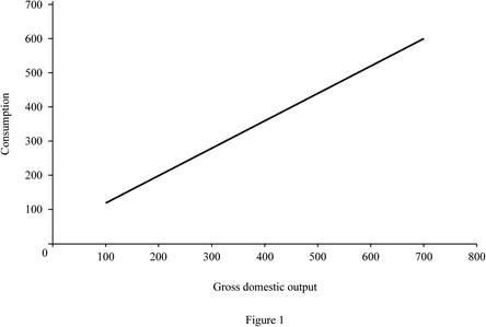
In Figure 1, the horizontal axis measures the gross domestic output and the vertical axis measures the consumption level.
Size of marginal propensity to consume (MPC) can be calculated as follows.
The size of marginal propensity to consume is 0.8.
Concept introduction:
Consumption schedule: Consumption schedule refers to the quantity of consumption at different levels of income.
Marginal propensity to consume (MPS): Marginal propensity to consume refers to the sensitivity of change in the consumption level due to the changes occurred in the income level.
Sub part (b):
Disposable income, tax rate, consumption schedule, marginal propensity to consume and multiplier.
Sub part (b):
Explanation of Solution
Disposable income (DI) can be calculated by using the following formula.
Substitute the respective values in Equation (1) to calculate the disposable income at the level of GDP $100.
Disposable income at the level of GDP $100 is $90.
Tax rate can be calculated by using the following formula.
Substitute the respective values in Equation (2) to calculate the tax rate at the level of GDP $100.
Tax rate at the level of GDP is 10%.
New consumption level can be calculated by using the following formula.
Substitute the respective values in Equation (3) to calculate the disposable income at the level of GDP $100. Since, the tax payment is equal amount of decrease in consumption for all the levels of GDP. The decreasing consumption for increasing $10 is assumed to be $8.
New consumption is $112.
Table -2 shows the values of disposable income, new consumption level after tax and the tax rate that are obtained by using Equations (1), (2) and (3).
Table -2
| Gross domestic product | Tax | DI | New consumption | Tax rate |
| 100 | 10 | 90 | 112 | 10% |
| 200 | 10 | 190 | 192 | 5% |
| 300 | 10 | 290 | 272 | 3.33% |
| 400 | 10 | 390 | 352 | 2.5% |
| 500 | 10 | 490 | 432 | 2% |
| 600 | 10 | 590 | 512 | 1.67% |
| 700 | 10 | 690 | 592 | 1.43% |
Size of marginal propensity to consume (MPC) can be calculated as follows.
The size of marginal propensity to consume is 0.8.
Multiplier: Multiplier refers to the ratio of change in the real GDP to the change in initial consumption, at a constant price rate. Multiplier is positively related to the marginal propensity to consumer and negatively related with the marginal propensity to save. Multiplier can be evaluated using the following formula:
Since the value of MPC remains the same for part (a) and part (b), there is no change in the value of multiplier. The value of multiplier is 5
Figure -2 illustrates the level of consumption at different level of gross domestic product (GDP) for lump sum tax (Regressive tax).
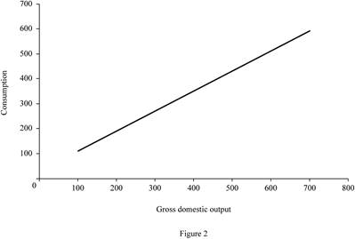
In Figure -2, the horizontal axis measures the gross domestic output and the vertical axis measures the consumption level.
Concept introduction:
Consumption schedule: Consumption schedule refers to the quantity of consumption at different levels of income.
Marginal propensity to consume (MPS): Marginal propensity to consume refers to the sensitivity of change in the consumption level due to the changes occurred in the income level.
Multiplier: Multiplier refers to the ratio of change in the real GDP to the change in initial consumption at constant price rate. Multiplier is positively related to the marginal propensity to consumer and negatively related with the marginal propensity to save.
Sub part (c):
Tax amount, consumption schedule, marginal propensity to consume and multiplier.
Sub part (c):
Explanation of Solution
Tax amount can be calculated by using the following formula.
Substitute the respective values in Equation (4) to calculate the tax amount at $100 GDP.
Tax amount is $10.
Table -3 shows the values of disposable income, new consumption level after tax and the tax rate that are obtained by using Equations (1), (2), (3) and (4). The change in tax amount is differing for different levels of GDP. The decreasing consumption for increasing each $10 is assumed to be $8 (Thus, if the tax payment is $30, then the consumption decreases by $24
Table -3
| Gross domestic product | Tax | DI | New consumption | Tax rate |
| 100 | 10 | 90 | 112 | 10% |
| 200 | 20 | 180 | 184 | 10% |
| 300 | 30 | 270 | 256 | 10% |
| 400 | 40 | 360 | 328 | 10% |
| 500 | 50 | 450 | 400 | 10% |
| 600 | 60 | 540 | 472 | 10% |
| 700 | 70 | 630 | 544 | 10% |
Multiplier: Multiplier refers to the ratio of change in the real GDP to the change in initial consumption, at a constant price rate. Multiplier is positively related to the marginal propensity to consumer and negatively related with the marginal propensity to save. Multiplier can be evaluated using the following formula:
Since the value of MPC different for part (a) and part (c), the value of multiplier for both the part is different. The value of multiplier is 3.57
Figure -3 illustrates the level of consumption at different level of gross domestic product (GDP) for proportional tax.
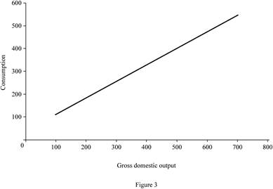
In Figure -3, the horizontal axis measures the gross domestic output and the vertical axis measures the consumption level.
Concept introduction:
Consumption schedule: Consumption schedule refers to the quantity of consumption at different levels of income.
Marginal propensity to consume (MPS): Marginal propensity to consume refers to the sensitivity of change in the consumption level due to the changes occurred in the income level.
Multiplier: Multiplier refers to the ratio of change in the real GDP to the change in initial consumption at constant price rate. Multiplier is positively related to the marginal propensity to consumer and negatively related with the marginal propensity to save.
Sub part (d):
consumption schedule, marginal propensity to consume and multiplier.
Sub part (d):
Explanation of Solution
Marginal propensity to consume can be calculated by using the following formula.
Substitute the respective values in Equation (5) to calculate the MPC at $100 GDP.
The value of MPC is 0.72.
Table -4 shows the values of disposable income, new consumption level after tax and the tax rate that are obtained by using Equations (1), (2), (3), (4) and (5). The change in tax amount is differing for different levels of GDP. The decreasing consumption for increasing each $10 is assumed to be $8 (Thus, if the tax payment is $20, then the consumption decreases by $16
Table -3
| Gross domestic product | Tax | DI | New consumption | Tax rate | MPC |
| 100 | 0 | 100 | 120 | 0% | |
| 200 | 10 | 190 | 192 | 5% | 0.8 |
| 300 | 30 | 270 | 256 | 10% | 0.64 |
| 400 | 60 | 340 | 312 | 15% | 0.56 |
| 500 | 100 | 400 | 360 | 20% | 0.48 |
| 600 | 150 | 450 | 400 | 25% | 0.4 |
| 700 | 210 | 490 | 432 | 30% | 0.32 |
Multiplier: Multiplier refers to the ratio of change in the real GDP to the change in initial consumption, at a constant price rate. Multiplier is positively related to the marginal propensity to consumer and negatively related with the marginal propensity to save.
Multiplier value is differing for each level of GDP. When the tax rate increases, it reduces the value of MPC. Since the value of MPC decreases, the value of multiplier will also decrease.
Figure 4 illustrates the level of consumption at different level of gross domestic product (GDP) for progressive tax.
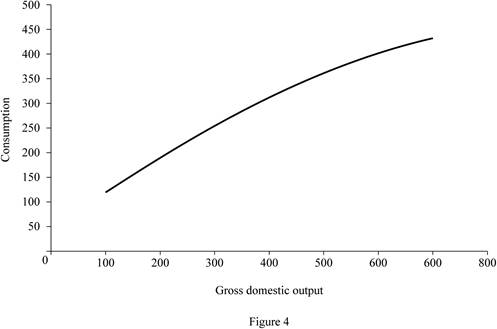
In Figure 4, the horizontal axis measures the gross domestic output and the vertical axis measures the consumption level.
Concept introduction:
Consumption schedule: Consumption schedule refers to the quantity of consumption at different levels of income.
Marginal propensity to consume (MPS): Marginal propensity to consume refers to the sensitivity of change in the consumption level due to the changes occurred in the income level.
Multiplier: Multiplier refers to the ratio of change in the real GDP to the change in initial consumption at constant price rate. Multiplier is positively related to the marginal propensity to consumer and negatively related with the marginal propensity to save.
Sup part (e):
Marginal propensity to consume and multiplier.
Sup part (e):
Explanation of Solution
Figure 1, Figure 2, Figure 3 and Figure 4 reveals that the proportional and progressive tax system reduces the value of MPC, so that the value of multiplier also decreases. The regressive tax system (Lump sum tax) does not alter the MPC. Since there is no change in the MPC, the multiplier remains the same.
Concept introduction:
Marginal propensity to consume (MPS): Marginal propensity to consume refers to the sensitivity of change in the consumption level due to the changes occurred in the income level.
Progressive tax: Progressive tax refers to the higher income people paying higher tax amount than the lower income people.
Proportional tax: Proportional tax rate refers to the fixed tax rate regardless of income and the tax rate and is the same for all levels of income.
Regressive tax: Regressive tax refers to the higher income people paying lower percentage of tax amount and lower income people paying higher percentage of tax amount.
Multiplier: Multiplier refers to the ratio of change in the real GDP to the change in initial consumption at constant price rate. Multiplier is positively related to the marginal propensity to consumer and negatively related with the marginal propensity to save.
Want to see more full solutions like this?
Chapter 13 Solutions
Macroeconomics: Principles, Problems, & Policies

- 6 Suppose a closed economy with no government spending or taxing initially. Suppose also that intended investment is equal to 100 and the aggregate consumption function is given by C = 250 + 0.75Y. And suppose that, if at full employment, the economy would produce an output and income of 3500 By how much would the government need to raise spending (G) to bring the economy to full employment? (round your answer to the nearest whole value)arrow_forward#wk4-10 Suppose that the investment demand curve in a certain economy is such that investment declines by $120 billion for every 1 percentage point increase in the real interest rate. Also, suppose that the investment demand curve shifts rightward by $170 billion at each real interest rate for every 1 percentage point increase in the expected rate of return from investment.If stimulus spending (an expansionary fiscal policy) by government increases the real interest rate by 2 percentage points, but also raises the expected rate of return on investment by 1 percentage point, how much investment, if any, will be crowded out?$ billionarrow_forwardSuppose that the investment demand curve in a certain economy is such that investment declines by $110 billion for every 1 percentage point increase in the real interest rate. Also, suppose that the investment demand curve shifts rightward by $170 billion at each real interest rate for every 1 percentage point increase in the expected rate of return from investment. If stimulus spending (an expansionary fiscal policy) by government increases the real interest rate by 2 percentage points, but also raises the expected rate of return on investment by 1 percentage point, how much investment, if any, will be crowded out? Note:- Do not provide handwritten solution. Maintain accuracy and quality in your answer. Take care of plagiarism. Answer completely. You will get up vote for sure.arrow_forward
- 7 Consider a model in which an individual lives only two periods. This person has diminishing marginal utility of consumption and receives an income of $20,000 in period 1 and an income of $5,000 in period 2. The private interest rate is 10 percent per period, and this person can borrow or lend money at this rate. Also assume that this person intends to consume all of his income over his lifetime. a. Give a hypothetical numerical example of what a person’s optimal consumption would be over these two periods. In answering this question, what assumptions did you make?arrow_forward7 Suppose a closed economy with no government spending which in equilibrium is producing an output and income of 1100. Suppose also that the marginal propensity to consume is 0.80, and that, if at full employment, the economy would produce an output and income of 3850 By how much would the government need to cut taxes (T) to bring the economy to full employment? (round your answer to the nearest whole value)arrow_forwardSuppose that consumer spending initially rises by $5 billion for every 1 percent rise in household wealth and that investment spending initially rises by $20 billion for every 1 percentage point fall in the real interest rate. Also assume that the economy�s multiplier is 3. If household wealth falls by 6 percent because of declining house values, and the real interest rate falls by 2 percentage points, in what direction and by how much will the aggregate demand curve initially shift at each price level? The aggregate demand curve will shift_____ by $____ billion. In what direction and by how much will it eventually shift? The aggregate demand curve will shift_____ by $____ billion..arrow_forward
- 9. True or false? If the statement is false, explain why: LO4 a. An internally held public debt is like a debt of the left hand owed to the right hand. b. The Federal Reserve and federal government agencies hold more than half the public debt. c. As a percentage of GDP, the federal debt held by the public was smaller in 2010 than it was in 1990. d. As a percentage of GDP, the total U.S. public debt is the highest such debt among the world’s advanced industrial nations.arrow_forward7 Suppose that the government increases its expenditure on goods and services by $100 billion and pays for these goods and services by raising autonomous taxes by $100 billion. What is the effect on aggregate demand and real GDP of each change individually and of the two combinedarrow_forward1.In Figure 1, when disposable income is 0, how much is consumption, saving, autonomous consumption, and induced consumption? 2.In Figure 1, when disposable income is 2500, how much is consumption, saving, autonomous consumption, and induced consumption? 3.In Figure 1, when disposable income is 4,000, how much is the consumption, savings, autonomous consumption and induced consumption?arrow_forward
- 2. Suppose that consumption equals $500 billion when the disposable income is $0 and that each increase of $100 billion in disposable income causes consumption to increase by $70 billion. a. Draw a graph of the consumption function using this information. The axes must be labeled correctly, and the consumption function should have at least two points on the graph (correct coordinates). b. What is the Marginal Propensity to Consume in this economy? How did you arrive at your answer? Please show your work. Note:- Do not provide handwritten solution. Maintain accuracy and quality in your answer. Take care of plagiarism. Answer completely. You will get up vote for sure.arrow_forward5 3. permanent Income Hypothesis a) suppose that beta=.9 and R= 2222 (that is ~22%). For an individual who acts according to the PIH, will their consumption next period be higher than current consumption or lower? b) What is the main crucial difference between the Keynesian Consumption function and the consumption function derived from the PIH (or Lifetime Income Hypothesis)? c) If Present Value of future income stream is 500,000 and a person has a beta of.8, how much will their consumption go up today if only today's income increases by 1000? How much will their consumption increase (approximately) if their income goes up by 1000 in all periods?arrow_forward3. Assume that initially G is $300 and equilibrium real GDP is $5000. If the multiplier is 5, what would be the new equilibrium level of GDP if Government expenditures increase to $600.arrow_forward

 Principles of Economics (12th Edition)EconomicsISBN:9780134078779Author:Karl E. Case, Ray C. Fair, Sharon E. OsterPublisher:PEARSON
 Engineering Economy (17th Edition)EconomicsISBN:9780134870069Author:William G. Sullivan, Elin M. Wicks, C. Patrick KoellingPublisher:PEARSON
 Principles of Economics (MindTap Course List)EconomicsISBN:9781305585126Author:N. Gregory MankiwPublisher:Cengage Learning
 Managerial Economics: A Problem Solving ApproachEconomicsISBN:9781337106665Author:Luke M. Froeb, Brian T. McCann, Michael R. Ward, Mike ShorPublisher:Cengage Learning
 Managerial Economics & Business Strategy (Mcgraw-...EconomicsISBN:9781259290619Author:Michael Baye, Jeff PrincePublisher:McGraw-Hill Education