Concept explainers
Videos
a.
Identify and explain whichof the given modelscan be recommended.
a.
Answer to Problem 66SE
The model with 2 predictors and the model with 3 predictors can be recommended for predicting the pH before addition of dyes.
Explanation of Solution
Given info:
The MINITAB output shows the best regression option for the data predicted for pH before the addition of dyes using carpet density, carpet weight, dye weight, dye weight as a percentage of carpet and pH after addition of dyes.
Justification:
Mallows
It is used to assess the fit of regression model where the aim to find the best subset of predictors. A relatively small value of
By observing the mallows
By examining the models with three variables,
Hence, the model with two predictorsnamely dye weight and pH after addition of dyes could be considered as a best model subset for predicting pH before the addition of dyes.
Also, a second option would be the model with three predictorsnamely carpet weight, dye weight and pH after addition of dyes could be considered as a best model subset for predicting pH before the addition of dyes.
b.
Test whether the model suggests a useful linear relationship between pH before the addition of dyes and at least one of the predictors.
b.
Answer to Problem 66SE
There is sufficient evidence to conclude that the there is a use of linear relationship between pH before the addition of dyes and at least one of the predictors dye weight and pH after the addition of dyes.
Explanation of Solution
Given info:
The MINITAB output for predicting the pH before the addition of dyes using the dye weight
Calculation:
The test hypotheses are given below:
Null hypothesis:
That is, there is no use of linear relationship between pH before the addition of dyes and the predictors dye weightand pH after the addition of dyes.
Alternative hypothesis:
That is, there is a use of linear relationship between pH before the addition of dyes and at least one of the predictors dye weightand pH after the addition of dyes.
Conclusion:
The P-value is 0.000 and the level of significance is 0.001.
The P-value is lesser than the level of significance.
That is
Thus, the null hypothesis is rejected.
Hence, there is sufficient evidence to conclude that there is a use of linear relationship between pH before the addition of dyes and at least one of the predictors dye weight and pH after the addition of dyes.
c.
Explain whether either one of the predictors could be eliminated from the model given that the other predictor is retained.
c.
Answer to Problem 66SE
No, either one of the predictors could not be eliminated from the model given that the other predictor is retained.
Explanation of Solution
Calculation:
For variable
Testing the hypothesis:
Null hypothesis:
That is, there is no use of linear relationship between pH before the addition of dyes and dye weightgiven that pH after addition of dyes was retained in the model.
Alternative hypothesis:
That is, there is a use of linear relationship between pH before the addition of dyes and dye weightgiven that pH after addition of dyes was retained in the model.
From the MINITAB output it can be observed that the P-value corresponding to the t statistic of
Conclusion:
The P-value is 0.000 and the level of significance is 0.001.
The P-value is lesser than the level of significance.
That is
Thus, the null hypothesis is rejected.
Hence, there is sufficient evidence to conclude that there is a use of linear relationship between pH before the addition of dyes and dye weight given that pH after addition of dyes was retained in the model.
For variable
Testing the hypothesis:
Null hypothesis:
That is, there is no use of linear relationship between pH before the addition of dyes and pH after addition of dyes given that dye weight was retained in the model.
Alternative hypothesis:
That is, there is a use of linear relationship between pH before the addition of dyes and pH after addition of dyes given that dye weight was retained in the model.
From the MINITAB output it can be observed that the P-value corresponding to the t statistic of
Conclusion:
The P-value is 0.000 and the level of significance is 0.001.
The P-value is lesser than the level of significance.
That is
Thus, the null hypothesis is rejected.
Hence, there is sufficient evidence to conclude that there is a use of linear relationship between pH before the addition of dyes and pH after addition of dyes given that dye weight was retained in the model.
Justification:
From the analysis it can be concluded that none of the variables can be eliminated from the model given that the other variable is already present in the model.
d.
Calculate and interpret the 95% confidence interval for the two predictors.
d.
Answer to Problem 66SE
The 95% confidence interval for the estimated slope coefficient
(–0.0000684, –0.0000244).
The 95% confidence interval for the estimated slope coefficient
Explanation of Solution
Calculation:
The 95% confidence interval is calculated using the formula:
The confidence interval is calculated using the formula:
Where,
n is the total number of observations.
k is the total number of predictors in the model.
Critical value:
Software procedure:
Step-by-step procedure to find the critical value is given below:
- Click on Graph, select View Probability and click OK.
- Select t, enter 111 as Degrees of freedom, inShaded Area Tab select Probability under Define Shaded Area By and choose Both tails.
- Enter Probability value as 0.05.
- Click OK.
Output obtained from MINITAB is given below:
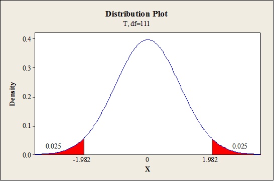
The 95% confidence interval for
Thus, the 95% confidence interval for the estimated slope coefficient
(–0.0000684, –0.0000244).
The 95% confidence interval for
Thus, the 95% confidence interval for the estimated slope coefficient
(0.6417,0.8325).
Interpretation:
For the variable
For one unit increase in the dye weight, it is 95% confident that the estimated value of pH before addition of dyes would decrease between–0.00000684 and–0.0000244 given that pH after addition of dyes is fixed constant.
For the variable
For one unit increase in the pH after the addition of dyes it is 95% confident that the estimated value of pH before addition of dyes would increase between 0.6417 and 0.8325 given that dye weight is fixed constant.
e.
Calculate and interpret the 95% confidence interval for the average value of pH before the addition of dyes when the dye weight and pH after the addition of dyes takes 1,000 and 6, respectively.
e.
Answer to Problem 66SE
The 95% confidence interval for the average value of pH before the addition of dyes when the dye weight and pH after the addition of dyes takes 1,000 and 6, respectively is (5.250, 5.383)
Explanation of Solution
Given info:
The estimated standard deviation for predicting the pH before the addition of dyes when the dye weight and pH after the addition of dyes takes 1,000 and 6 is 0.0336.
Calculation:
The average value of pH before the addition of dyes when the dye weight and pH after the addition of dyes takes 1,000 and 6 is calculated as follows:
Thus, the average value of pH before the addition of dyes when the dye weight and pH after the addition of dyes takes 1,000 and 6 is 5.316.
95% confidence interval for the true response:
The confidence interval is calculated using the formula:
Where,
n is the total number of observations.
k is the total number of predictors in the model.
Critical value:
Software procedure:
Step-by-step procedure to find the critical value is given below:
- Click on Graph, select View Probability and click OK.
- Select t, enter 111 as Degrees of freedom, in Shaded Area Tab select Probability under Define Shaded Area By and choose Both tails.
- Enter Probability value as 0.05.
- Click OK.
Output obtained from MINITAB is given below:
The 95% confidence interval is given below:
Thus, the 95% confidence interval for the average value of pH before the addition of dyes when the dye weight and pH after the addition of dyes takes 1,000 and 6 is (5.250,5.383).
Interpretation:
It is 95% confident that average value of pH before the addition of dyes when the dye weight and pH after the addition of dyes takes 1,000 and 6 would lie between 5.250 and 5.383.
Want to see more full solutions like this?
Chapter 13 Solutions
Probability and Stats. for Engineering.. (Looseleaf)


- Years of Work Experience and number of Job Offers of 10 job-seekers were as follows: Work Exp. 4 2 5 3 7 12 2 5 4 9 No. of Offers 7 1 8 4 13 19 3 11 9 15 a. Fit the regression equation of No. of Job Offers on Years of Work Experience. b. What will be the predicted number of offers for an applicant with 6 years of experience? c. Verify the relationship between the number of job offers and years of work experience using at least two relevant methodsarrow_forwardA researcher notes that, in a certain region, a disproportionate number of software millionaires were born around the year 1955. Is this a coincidence, or does birth year matter when gauging whether a software founder will besuccessful? The researcher investigated this question by analyzing the data shown in the accompanying table. Complete parts a through c below. a. Find the coefficient of determination for the simple linear regression model relating number (y) of software millionaire birthdays in a decade to total number (x) of births in the region. Interpret the result. The coefficient of determination is 1.___? (Round to three decimal places as needed.) This value indicates that 2.____ of the sample variation in the number of software millionaire birthdays is explained by the linear relationship with the total number of births in the region. (Round to one decimal place as needed.) b. Find the coefficient of determination for the simple linear regression model…arrow_forwardA researcher developed a regression model to predict the cost of a meal based on the summated rating (sum of ratings for food, decor,and service) and the cost per meal for 12 restaurants. The results of the study show that b1=1.4379 and Sb1=0.1397. a. At the 0.05 level of significance, is there evidence of a linear relationship between the summated rating of a restaurant and the cost of a meal? b. Construct a 95% confidence interval estimate of the population slope, β1. a. Determine the hypotheses for the test. Choose the correct answer below. A. H0: β1=0 H1: β1≠0 B. H0: β0≤0 H1: β0>0 C. H0: β1≤0 H1: β1>0 D. H0: β0≥0 H1: β0<0 E. H0: β1≥0 H1: β1<0 F. H0: β0=0 H1: β0≠0 Compute the test statistic. The test statistic is ? (Round to two decimal places as needed.) Determine the critical value(s). The critical value(s) is(are) ? (Use a comma to separate answers as needed.…arrow_forward
- consider the coefficient estimates of the following market model linear regression of general motors (gm) on the S&P500 market returns coefficient estimate std error tvalue pr(>ItI) intercept 0.005860 0.0003704 1.582 0.12412 sp500 0.0904753 0.266702 3.392 0.00196 The number of observations is 32.At the 1% significance level, what is the (1)test statistic value,(2) the critical values (3) decision regarding the null hypothesis that the beta coefficient on the market returns is equal to 1.61arrow_forwardA newspaper used an estimated regression equation to describe the relationship between y = error percentage for subjects reading a four-digit liquid crystal display and the independent variables x1 = level of backlight, x2 = character subtense, x3 = viewing angle, and x4 = level of ambient light. From a table given in the article, SSRegr = 21.6, SSResid = 22, and n = 30. What is the value of the test statistic F What is the P-value What is r2 What is Searrow_forwardThe systolic blood pressure dataset (in the third sheet of the spreadsheet linked above) contains the systolic blood pressure and age of 30 randomly selected patients in a medical facility. What is the equation for the least square regression line where the independent or predictor variable is age and the dependent or response variable is systolic blood pressure? Y=__________ X + ______________ Patient 7 is 67 years old and has a systolic blood pressure of 170 mm Hg. What is the residual? __________ mm Hg Is the actual value above, below, or on the line? What is the interpretation of the residual? (difference in actual &predicated bp, difference in age, the amount of systolic changes)arrow_forward
- Given the estimated least square regression line y=2.48+1.63x, and the coefficient of determination of 0.81, What is the value of correlation coefficient?arrow_forwardA study was conducted to see whether heart rate (y) on swimmers linearly related to their age (x1) and swimming time for 2000 meters (x2). A random sample of ten swimmers was selected and the result is shown in the following Microsoft Excel output. (a)Interpret the value of R2 from the output. (b)Conduct a hypothesis test to test whether the linear regression model is fit or not using a = 0.05. (c)Calculate the 95% confidence interval for the coefficient value for age.arrow_forwardThe following output was obtained from a multiple regression analysis. Analysis of variance SOURCE DF SS MS Regression 5 100 20 Residual Error 20 40 2 Total 25 140 Predictor Coefficient SE Coefficient t Constant 3.00 1.50 2.00 x1 4.00 3.00 1.33 x2 3.00 0.20 15.00 x3 0.20 0.05 4.00 x4 −2.50 1.00 −2.50 x5 3.00 4.00 0.75 Conduct a global test of hypothesis H0: β1 = β2 = β3 = β4 = β5 = 0; H1: Not all β's are 0 at the 0.05 significance level. d-1. State the decision rule. (Round your answer to 2 decimal places.) Reject H0 if F> d-2. What is the computed value of F? (Round your answer to 1 decimal place.) Value of F d-3. Determine whether any of the regression coefficients are significant. ----------------Reject H0 Atleast One regression Coefficient is---------------- Accept Zero…arrow_forward
- An econometrician suspects that the residuals of her model might be autocorrelated. Explain the steps involved in testing this theory using the Durbin–Watson (DW) testarrow_forwardThe calories and sugar content per serving size of ten brands of breakfast cereal are fitted with a least squares regression line with computer outputs:arrow_forwardWhich of the multivariate regression parameters listed below would be best interpreted as: the predicted value on the dependent variable when all of the independent variables in the model are equal to zero. a b1 X1 R2arrow_forward
 MATLAB: An Introduction with ApplicationsStatisticsISBN:9781119256830Author:Amos GilatPublisher:John Wiley & Sons Inc
 Probability and Statistics for Engineering and th...StatisticsISBN:9781305251809Author:Jay L. DevorePublisher:Cengage Learning
 Statistics for The Behavioral Sciences (MindTap C...StatisticsISBN:9781305504912Author:Frederick J Gravetter, Larry B. WallnauPublisher:Cengage Learning
 Elementary Statistics: Picturing the World (7th E...StatisticsISBN:9780134683416Author:Ron Larson, Betsy FarberPublisher:PEARSON
 The Basic Practice of StatisticsStatisticsISBN:9781319042578Author:David S. Moore, William I. Notz, Michael A. FlignerPublisher:W. H. Freeman
 Introduction to the Practice of StatisticsStatisticsISBN:9781319013387Author:David S. Moore, George P. McCabe, Bruce A. CraigPublisher:W. H. Freeman