
Concept explainers
Videos
The accompanying data on y 5 energy output (W) and x 5 temperature difference (°K) was provided by the authors of the article “Comparison of Energy and Exergy Efficiency for Solar Box and Parabolic Cookers” (J. of Energy Engr., 2007: 53–62). The article’s authors fit a cubic regression model to the data. Here is Minitab output from such a fit.
| x | 23.20 | 23.50 | 23.52 | 24.30 | 25.10 | 26.20 | 27.40 | 28.10 | 29.30 | 30.60 | 31.50 | 32.01 |
| y | 3.78 | 4.12 | 4.24 | 5.35 | 5.87 | 6.02 | 6.12 | 6.41 | 6.62 | 6.43 | 6.13 | 5.92 |
| x | 32.63 | 33.23 | 33.62 | 34.18 | 35.43 | 35.62 | 36.16 | 36.23 | 36.89 | 37.90 | 39.10 | 41.66 |
| y | 5.64 | 5.45 | 5.21 | 4.98 | 4.65 | 4.50 | 4.34 | 4.03 | 3.92 | 3.65 | 3.02 | 2.89 |
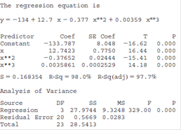
a. What proportion of observed variation in energy output can be attributed to the model relationship?
b. Fitting a quadratic model to the data results in R2 = .780. Calculate adjusted R2 for this model and compare to adjusted R2 for the cubic model.
c. Does the cubic predictor appear to provide useful information about y over and above that provided by the linear and quadratic predictors? State and test the appropriate hypotheses.
d. When x = 30,
e. Interpret the hypotheses

Trending nowThis is a popular solution!

Chapter 13 Solutions
Student Solutions Manual for Devore's Probability and Statistics for Engineering and the Sciences, 9th


- The following table provides values of the function f(x,y). However, because of potential; errors in measurement, the functional values may be slightly inaccurately. Using the statistical package included with a graphical calculator or spreadsheet and critical thinking skills, find the function f(x,y)=a+bx+cy that best estimate the table where a, b and c are integers. Hint: Do a linear regression on each column with the value of y fixed and then use these four regression equations to determine the coefficient c. x y 0 1 2 3 0 4.02 7.04 9.98 13.00 1 6.01 9.06 11.98 14.96 2 7.99 10.95 14.02 17.09 3 9.99 13.01 16.01 19.02arrow_forwardRespiratory Rate Researchers have found that the 95 th percentile the value at which 95% of the data are at or below for respiratory rates in breath per minute during the first 3 years of infancy are given by y=101.82411-0.0125995x+0.00013401x2 for awake infants and y=101.72858-0.0139928x+0.00017646x2 for sleeping infants, where x is the age in months. Source: Pediatrics. a. What is the domain for each function? b. For each respiratory rate, is the rate decreasing or increasing over the first 3 years of life? Hint: Is the graph of the quadratic in the exponent opening upward or downward? Where is the vertex? c. Verify your answer to part b using a graphing calculator. d. For a 1- year-old infant in the 95 th percentile, how much higher is the walking respiratory rate then the sleeping respiratory rate? e. f.arrow_forwardIf your graphing calculator is capable of computing a least-squares sinusoidal regression model, use it to find a second model for the data. Graph this new equation along with your first model. How do they compare?arrow_forward
- Olympic Pole Vault The graph in Figure 7 indicates that in recent years the winning Olympic men’s pole vault height has fallen below the value predicted by the regression line in Example 2. This might have occurred because when the pole vault was a new event there was much room for improvement in vaulters’ performances, whereas now even the best training can produce only incremental advances. Let’s see whether concentrating on more recent results gives a better predictor of future records. (a) Use the data in Table 2 (page 176) to complete the table of winning pole vault heights shown in the margin. (Note that we are using x=0 to correspond to the year 1972, where this restricted data set begins.) (b) Find the regression line for the data in part ‚(a). (c) Plot the data and the regression line on the same axes. Does the regression line seem to provide a good model for the data? (d) What does the regression line predict as the winning pole vault height for the 2012 Olympics? Compare this predicted value to the actual 2012 winning height of 5.97 m, as described on page 177. Has this new regression line provided a better prediction than the line in Example 2?arrow_forwardFind the equation of the regression line for the following data set. x 1 2 3 y 0 3 4arrow_forwardA particular article used a multiple regression model with the following four independent variables. y = error percentage for subjects reading a four-digit liquid crystal displayx1 = level of backlight (from 0 to 122 cd/m)x2 = character subtense (from .025 to 1.34)x3 = viewing angle (from 0 to 60)x4 = level of ambient light (from 20 to 1500 lx) The model equation suggested in the article is given below. (a) Assume that this is the correct equation. What is the mean value of y when x1 = 30, x2 = 0.6, x3 = 50 and x4 = 150?(b) What mean error percentage is associated with a backlight level of 40, character subtense of 0.6, viewing angle of 20, and ambient light level of 30?arrow_forward
- A researcher records age in years (x) and systolic blood pressure (y) for volunteers. They perform a regression analysis was performed, and a portion of the computer output is as follows: ŷ = 3.3 +12.7x Coefficients (Intercept) X Estimate Std. Error Test statistic O Ho: B₁: = 0 Ha: B₁ 0 O Ho: B₁ = 0 Ha: B₁ 0 12.7 2.2 6.4 1.5 1.98 P-value Specify the null and the alternative hypotheses that you would use in order to test whether a positive linear relationship exists between x and y. 0.08 0.03arrow_forwarda) We conduct a regression of size on hhinc, owner, hhsize, hhsize2,and hhsize3. We do not include the constant. The regression output is reported in Table 3. Would you conclude that the home size increases with the household size? Interpret the sign and magnitude of the estimated coefficients of hhsize1, hhsize2, and hhsize3.arrow_forwardI need help with part b please. linear regression equation: y_hat = 6.6500 + 1.7000x table of temperatures versus converted sugars: Temperature, x Converted Sugar, y 1 8.2 1.1 8.1 1.2 8.7 1.3 9.9 1.4 9.6 1.5 8.7 1.6 8.2 1.7 10.6 1.8 9.3 1.9 9.2 2 10.7arrow_forward
- The data set was obtained from 21 days of operation of a plant for the oxidation of ammonia to nitric acid. It is desired to fit a multiple linear regression model to predict Y = stack loss which is 10 times the percentage of the ingoing ammonia to the plant that escapes from the absorption column unabsorbed, as Y = Bo + B1Xair.flow + B2 water.temp + B3 xacid.conc Air.Flow represents the rate of operation of the plant. Water.Temp is the temperature of cooling water circulated through coils in the absorption tower. Acid.Conc is the concentration of the acid circulating, minus 50, times 10. This is the result of the best subsets regression. |Summary of best subsets, variable(s): stack.loss (stt 151astackloss) Adjusted R square and standardized regression coefficients for each submodel Adjusted R square 0.898623 No. of Effects Air. Flow Water.Temp Acid.Conc. Subset No. 1 2 0.604950 0.402523 This is the result of the forward stepwise regression. Degr. of Freedom P to enter 0.000000 Effect…arrow_forwardCompute for the necessary linear regressions based on the given data. (can use Excel or Minitab for this) An article in the Tappi Journal (March, 1986) presented data on green liquor Na2S concentration (in grams per liter) and paper machine production (in tons per day). The data (read from a graph) are shown as follows: (a) Fit a simple linear regression model with y green liquor Na2S concentration and x production. Draw a scatter diagram of the data and the resulting least squares fitted model.(b) Find the fitted value of y corresponding to x = 910 and the associated residual.arrow_forwardA researcher records age in years (x) and systolic blood pressure (y) for volunteers. They perform a regression analysis was performed, and a portion of the computer output is as follows: ŷ = 4.3 14.9x Coefficients (Intercept) X Estimate St 4.3 Ho: B₁ = 0 Ha: B₁ > 0 B1 O Ho: B₁ Ha: B₁ <0 = 0 14.9 B1 O Ho: B₁ = 0 0 Ha: B1 Std. Error Test statistic P-value 2.9 5.1 1.48 Specify the null and the alternative hypotheses that you would use in order to test whether a negative linear relationship exists between x and y. 2.92 0.08 0.01arrow_forward
 College AlgebraAlgebraISBN:9781305115545Author:James Stewart, Lothar Redlin, Saleem WatsonPublisher:Cengage Learning
 Trigonometry (MindTap Course List)TrigonometryISBN:9781305652224Author:Charles P. McKeague, Mark D. TurnerPublisher:Cengage Learning
 Calculus For The Life SciencesCalculusISBN:9780321964038Author:GREENWELL, Raymond N., RITCHEY, Nathan P., Lial, Margaret L.Publisher:Pearson Addison Wesley,
 Algebra & Trigonometry with Analytic GeometryAlgebraISBN:9781133382119Author:SwokowskiPublisher:Cengage
 Algebra and Trigonometry (MindTap Course List)AlgebraISBN:9781305071742Author:James Stewart, Lothar Redlin, Saleem WatsonPublisher:Cengage Learning
 Functions and Change: A Modeling Approach to Coll...AlgebraISBN:9781337111348Author:Bruce Crauder, Benny Evans, Alan NoellPublisher:Cengage Learning