Concept explainers
Videos
Refer to the Real Estate data, which report information on homes sold in Goodyear, Arizona. Use the selling price of the home as the dependent variable and determine the regression equation with number of bedrooms, size of the house, center of the city, and number of bathrooms as independent variables.
- a. Use a statistical software package to determine the multiple regression equation. Discuss each of the variables. For example, are you surprised that the regression coefficient for distance from the center of the city is negative? How much does a garage or a swimming pool add to the selling price of a home?
- b. Determine the value of the Intercept.
- c. Develop a correlation matrix. Which independent variables have strong or weak
correlations with the dependent variable? Do you see any problems with multicollinearity? - d. Conduct the global test on the set of independent variables. Interpret.
- e. Conduct a test of hypothesis on each of the independent variables. Would you consider deleting any of the variables? If so, which ones?
- f. Rerun the analysis until only significant regression coefficients remain in the analysis. Identify these variables.
- g. Develop a histogram or a stem-and-leaf display of the residuals from the final regression equation developed in part (f). Is it reasonable to conclude that the normality assumption has been met?
- h. Plot the residuals against the fitted values from the final regression equation developed in part (f). Plot the residuals on the vertical axis and the fitted values on the horizontal axis.
a.
Find the multiple regression equation.
Explain each of the variables.
Answer to Problem 33DE
The multiple regression equation is as follows:
Explanation of Solution
Let y is dependent variable,
Where, y is the selling price of a house,
Step-by-step procedure to obtain the regression equation using MINITAB software:
- Choose Stat > Regression > Regression > Fit Regression Model.
- Under Responses, enter the column of Price.
- Under Continuous predictors, enter the columns of Bedrooms, Size, Center of the city and Bathrooms, pools and Garage.
- Click OK.
Output using MINITAB software is given below:
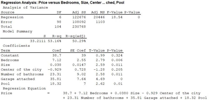
From the above output, the multiple regression equation is as follows:
The slope coefficients of bedrooms, size, and center of the city, bedrooms, pool and garage are 7.12, 0.0380, 0.929, 23.31, 18.32, and 35.18, respectively.
For each additional bedroom, the selling price of house will increase by $7,120 on average when all of the other variables are constant.
For each additional square foot of the size in the house, the price of the house will increase by $38.
For each additional mile away from the center of the city, the selling price of home decreases by $929.
For each additional bathroom, then the selling price of home will increase by $2,331 on average.
A house with a pool increases $1,832 to the selling price of the home and a house with garage will increase $3,581 to the selling price of a house.
b.
Find the value of intercept.
Answer to Problem 33DE
The value of intercept is $38.7.
Explanation of Solution
From Part (a) output, the value of intercept is $38.7.
The intercept value indicates the price for the home at the center of the city when all other factors are zero.
c.
Make the correlation matrix.
Find the independent variables those that have strong or weak correlations with the dependent variables.
Explain whether there are any problems with multicollinearity.
Explanation of Solution
Multicollinearity:
In a multiple regression model, when there is high correlation between two or more independent variables, then multicollinearity occurs.
Due to this multicollinearity the standard errors will be high and there will be no exact estimate of the partial regression coefficient. Moreover, there will be difficulty to measure the relative significance of independent variables.
Step-by-step procedure to obtain the correlation matrix using MINITAB software:
- Choose Stat > Basic Statistics > Correlation.
- Select the columns of Price, Size, Bedrooms, Bathrooms, Pool, and Garage under Variables tab.
- Click OK.
Output obtained using Minitab is as follows:
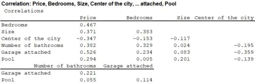
From the obtained output, there is a moderate correlation between the price and garage.
The variables price and distance from the center are negatively correlated. Thus, there is no strong correlation among the variables. The independent variables pool and size have weak correlation with the dependent variable.
It can be said that there is no high correlation among the independent variables. Thus, there is no multicollinearity among the independent variables.
d.
Conduct a global test on the set of the independent variables and interpret.
Explanation of Solution
The null and alternative hypotheses are stated below:
Null hypothesis:
That is, all the regression coefficients are equal to zero.
Alternative hypothesis:
From Part (a), the F test statistic value is 18.54 and the p-value is 0.000.
Decision rule:
- If
- Otherwise, failed to reject the null hypothesis.
Conclusion:
Consider the significance level as 0.05.
Here, the
That is, the p-value is less than the level of significance.
Therefore, reject the null hypothesis.
Hence, it can be concluded that all the regression coefficients are not equal to zero.
e.
Perform individual tests of each independent variable.
Explanation of Solution
For independent variable
Consider that
State the hypotheses:
Null hypothesis:
That is, there is no significant relationship between y and
Alternative hypothesis:
That is, there is significant relationship between y and
In the case of individual regression coefficient test, the t test statistic is defined as follows:
From Part (a), the t statistic value corresponding to
Consider the level of significance is
Decision rule:
- If
- Otherwise, failed to reject the null hypothesis.
Conclusion:
Here, the p-value corresponding to the “Bedrooms”
Hence,
That is, the p-value is less than the level of significance.
Therefore, reject the null hypothesis.
Hence, it can be concluded that there is significant relationship between y and
For independent variable
Consider that
State the hypotheses:
Null hypothesis:
That is, there is no significant relationship between y and
Alternative hypothesis:
That is, there is significant relationship between y and
From output in Part (a), the value of t-test statistic corresponding to
Conclusion:
Here, the p-value corresponding to the “Size”
The p-value is less than the level of significance.
That is, the
Therefore, reject the null hypothesis.
Hence, it can be concluded that there is a significant relationship between y and
For independent variable
Consider that
State the hypotheses:
Null hypothesis:
That is, there is no significant relationship between y and
Alternative hypothesis:
That is, there is significant relationship between y and
From the output in Part (a), the value of t test statistic corresponding to
Conclusion:
Here, the p-value corresponding to the “Center of the city”
The p-value is greater than the level of significance.
That is,
Therefore, fail to reject the null hypothesis.
Hence, it can be concluded that there is no significant relationship between y and
For independent variable
Consider that
State the hypotheses:
Null hypothesis:
That is, there is no significant relationship between y and
Alternative hypothesis:
That is, there is significant relationship between y and
From the output in Part (a), the value of t test statistic corresponding to
Conclusion:
Here, the p-value corresponding to the “bathrooms”
The p-value is less than the level of significance.
That is,
Therefore, reject the null hypothesis.
Hence, it can be concluded that there is a significant relationship between y and
For independent variable
Consider that
State the hypotheses:
Null hypothesis:
That is, there is no significant relationship between y and
Alternative hypothesis:
That is, there is significant relationship between y and
From the output in Part (a), the value of t test statistic corresponding to
Conclusion:
Here, the p-value corresponding to the “pool”
The p-value is less than the level of significance.
That is,
Therefore, reject the null hypothesis.
Hence, it can be concluded that there is a significant relationship between y and
For independent variable
Consider that
State the hypotheses:
Null hypothesis:
That is, there is no significant relationship between y and
Alternative hypothesis:
That is, there is significant relationship between y and
From the output in Part (a), the value of t test statistic corresponding to
Conclusion:
Here, the p-value corresponding to the “Garage”
The p-value is less than the level of significance.
That is,
Therefore, reject the null hypothesis.
Hence, it can be concluded that there is a significant relationship between y and
It is noticed that the p-value for the “center of the city” is greater than the level of significance. Thus, it is not a significant variable and it can be dropped from the model.
f.
Perform the regression analysis until only significant regression coefficients remain in the analysis.
Explanation of Solution
Step-by-step procedure to obtain the regression equation using MINITAB software:
- Choose Stat > Regression > Regression > Fit Regression Model.
- Under Responses, enter the column of Price.
- Under Continuous predictors, enter the columns of Bedrooms, Size, Bathrooms, Pools, and Garage.
- Click OK.
Output using MINITAB software is given below:
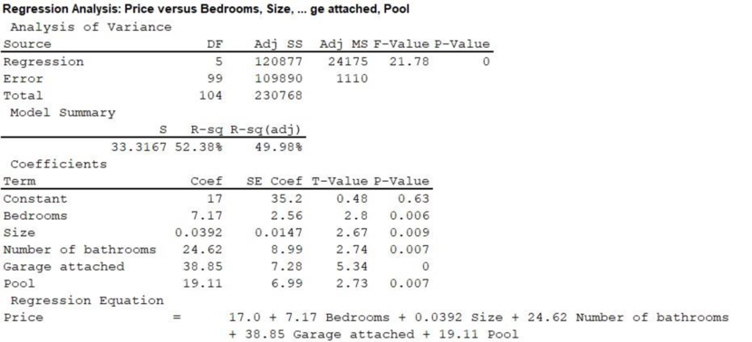
From the above output, the p-values for each of the independent variables are less than 0.05.
Thus, all the regression coefficients are significant for the dependent variable price. Even though the center of the city variable is dropped from the model, the coefficient of determination value is 0.5238 and it does not increase.
Therefore, the independent variables bedrooms, size, bathrooms, pool, and garage have significant effect on the price of house.
g.
Provide a histogram for the regression developed in Part (f).
Explain whether the residual follows normal distribution.
Explanation of Solution
Step-by-step procedure to obtain the regression equation using MINITAB software:
- Choose Stat > Regression > Regression > Fit Regression Model.
- Under Responses, enter the column of Price.
- Under Continuous predictors, enter the columns of Screen, Sharp, Samsung, and Sony.
- Choose Graphs.
- Under Residual plot select Histogram of residuals.
- Click OK.
The output obtained using MINITAB is as follows:
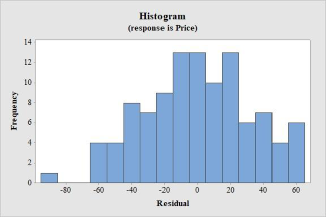
Assumption of normality from histogram:
- The majority of the observation in the middle and centered on the mean of 0.
- There are lower frequencies on the tails of the distributions.
According to the given histogram, most of the observations are centered on the mean of 0 and there are fewer frequencies on the tails of the distributions. Thus, it can be considered as roughly symmetric.
Hence, the residuals follow a normal distribution.
h.
Plot the residual plot for the regression developed in Part (f).
Explanation of Solution
Follow the same procedure mentioned in Part (g), one can get the following output:
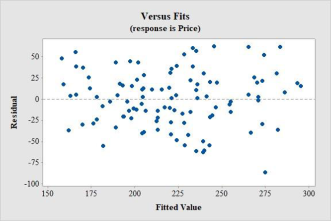
Assumption for residual analysis for the regression model:
- The plot of the residuals vs. the observed values of the predictor variable should fall roughly in a horizontal band and symmetric about the x-axis.
- For a normal probability plot, residuals should be roughly linear.
- There should not be any observable pattern.
According to the given residual plot, the points are roughly scattered and moreover, there is no particular pattern in the residual plot. A complete haphazard and random nature has been observed.
Want to see more full solutions like this?
Chapter 14 Solutions
Statistical Techniques in Business and Economics, 16th Edition


 Functions and Change: A Modeling Approach to Coll...AlgebraISBN:9781337111348Author:Bruce Crauder, Benny Evans, Alan NoellPublisher:Cengage Learning
 Glencoe Algebra 1, Student Edition, 9780079039897...AlgebraISBN:9780079039897Author:CarterPublisher:McGraw Hill
 Big Ideas Math A Bridge To Success Algebra 1: Stu...AlgebraISBN:9781680331141Author:HOUGHTON MIFFLIN HARCOURTPublisher:Houghton Mifflin Harcourt