Concept explainers
Videos
a.
Find the multiple regression equation.
Explain each of the variables.
Explain whether it is surprising that the regression coefficient for ERA is negative.
Explain whether the number of wins affected by whether the team plays in the National or the American League.
a.
Answer to Problem 34DE
The multiple regression equation is as follows:
Explanation of Solution
Let y is dependent variable,
Where, y is the number of win games, the team batting average (BA), number of stolen bases (SB), number of errors committed (Error), team earned run average (ERA), the number of home runs (HR) and whether the team plays in the American or the National League are denoted as
Step by step procedure to obtain the regression equation using MINITAB software:
- Choose Stat > Regression > Regression > Fit Regression Model.
- Under Responses, enter the column of Wins.
- Under Continuous predictors, enter the columns of BA, SB, Errors, ERA, HR, and League.
- Click OK.
Output using MINITAB software is given below:
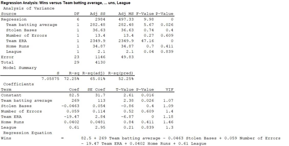
From the above output, the multiple regression equation is as follows:
For each additional point that the team batting average increases, the number of wins will increase by 0.269. Each additional stole base, the number of wins decrease by 0.0463. For each additional error committed by the team, the number of wins increases by 0.059. An additional increase on the ERA then the number of wins decrease by 19.47. For each additional home run will increase the number of wins by 0.0402. It is noticed that the variable league is coded as 0 and 1 for the National and the American respectively. Playing in the American League the number of wins is 0.61.
The negative regression coefficient for ERA indicates that as the team earned run average is decreased, then the number of Wins is increased and vice versa. There might be a negative correlation between ERA and the number of Wins. This is not surprising.
Consider that, the level of significance is
b.
Find the coefficient of determination (R-square).
b.
Answer to Problem 34DE
The coefficient of determination is 72.25%.
Explanation of Solution
From result of Part (a) output, the value of coefficient of determination (R-square) is 72.25%.
c.
Make the correlation matrix.
Find the independent variables those have strong or weak
Explain whether there is any problem of multicollinearity.
c.
Explanation of Solution
Multicollinearity:
In a multiple regression model, when there is high correlation between two or more independent variables, then multicollinearity occurs.
Due to this multicollinearity the standard errors will be high and there will be no exact estimate of the partial regression coefficient. Moreover, there will be difficulty to measure the relative significance of independent variables.
Step by step procedure to obtain the correlation matrix using MINITAB software is given below:
- Choose Stat > Basic Statistics > Correlation.
- Select the columns of BA, SB, Errors, ERA, HR, and League under Variables tab.
- Click OK.
The output obtained using Minitab is as follows:
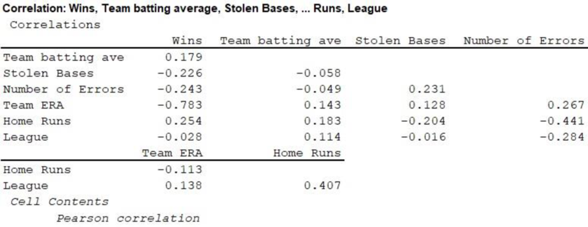
From the obtained output, ERA has strong correlation with dependent variable number of Wins. Whereas batting average, SB, Errors and Home runs have weak correlation with the number of wins. The correlation between League and the number of wins is –0.028. League does not appear to have any linear relationship with the number of wins.
It is noticed that there is no high correlation among the independent variables. Hence it can be concluded that, there is no presence of multicollinearity.
d.
Conduct a global test on the set of the independent variables and interpret.
d.
Explanation of Solution
The null and alternative hypotheses are stated below:
Null hypothesis:
That is, all the regression coefficients are equal to zero.
At least one of the regression coefficients is not equal to zero.
From Part (a), the F test statistic value is 9.98 and the p-value is 0.000.
Decision rule:
- If
- Otherwise failed to reject the null hypothesis.
Conclusion:
Consider the significance level as 0.05.
Here, the
That is, the p-value is less than the level of significance.
Therefore, reject the null hypothesis.
Hence, it can be concluded that all the regression coefficients are not equal to zero.
e.
Perform individual tests of each independent variable.
Explain whether any of the independent variables will be deleted.
e.
Explanation of Solution
For independent variable
Consider that
The null and alternative hypotheses are stated as follows:
Null hypothesis:
That is, there is no significant relationship between y and
Alternative hypothesis:
That is, there is significant relationship between y and
In case of individual regression coefficient test the t test statistic is defined as,
From Part (a) the t statistic value corresponding to
Consider the level of significance is
Conclusion:
Here, the p-value is less than the level of significance.
That is,
Therefore, reject the null hypothesis.
Thus, it can be concluded that there is significant relationship between y and
For independent variable
Consider that
The null and alternative hypotheses are stated as follows:
Null hypothesis:
That is, there is no significant relationship between y and
Alternative hypothesis:
That is, there is significant relationship between y and
From output in Part (a) the value of t test statistic corresponding to
Conclusion:
Here, the p-value is greater than the level of significance.
That is,
Hence by the rejection rule, fail to reject the null hypothesis.
Thus, it can be concluded that there is no significant relationship between y and
For independent variable
Consider that
State the hypotheses:
Null hypothesis:
That is, there is no significant relationship between y and
Alternative hypothesis:
That is, there is significant relationship between y and
From the output in Part (a) the value of t test statistic corresponding to
Conclusion:
Here, the p-value is greater than the level of significance
That is,
By the rejection, fail to reject the null hypothesis.
Hence, it can be concluded that there is no significant relationship between y and
For independent variable
Consider that
State the hypotheses:
Null hypothesis:
That is, there is no significant relationship between y and
Alternative hypothesis:
That is, there is significant relationship between y and
From the output in Part (a) the value of t test statistic corresponding to
Conclusion:
Here, the p-value is less than the level of significance
That is,
Therefore, reject the null hypothesis.
Hence, it can be concluded that there is a significant relationship between y and
For independent variable
Consider that
State the hypotheses:
Null hypothesis:
That is, there is no significant relationship between y and
Alternative hypothesis:
That is, there is significant relationship between y and
From the output in Part (a) the value of t test statistic corresponding to
Conclusion:
Here, the p-value is greater than the level of significance.
That is,
By the rejection rule, fail to reject the null hypothesis.
Hence, it can be concluded that there is no significant relationship between y and
For independent variable
Consider that
State the hypotheses:
Null hypothesis:
That is, there is no significant relationship between y and
Alternative hypothesis:
That is, there is significant relationship between y and
From the output in Part (a) the value of t test statistic corresponding to
Conclusion:
Here, the p-value is greater than the level of significance
That is,
By the rejection rule, fail to reject the null hypothesis.
Hence, it can be concluded that there is no significant relationship between y and
It is noticed that except the variables team batting average and team ERA, rest of the variables are insignificant. Therefore, the insignificant variables can be dropped from the model.
f.
Perform the
f.
Explanation of Solution
Step by step procedure to obtain the regression equation using MINITAB software:
- Choose Stat > Regression > Regression > Fit Regression Model.
- Under Responses, enter the column of Wins.
- Under Continuous predictors, enter the columns of BA, and ERA.
- Click OK
Output using MINITAB software is given below:
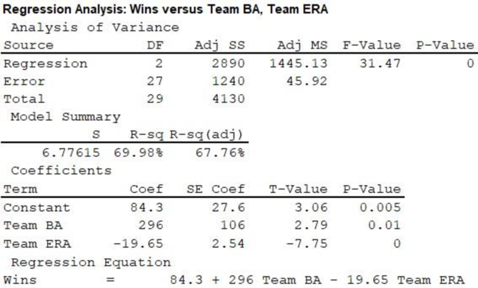
From the above output, the reduced regression model is
The p-values for each of the independent variables are less than 0.05. Therefore, the independent variables team BA and ERA have significant effect on the number of Wins.
g.
Provide a histogram for the regression developed in Part (f).
Explain whether the residual follows
g.
Explanation of Solution
Step by step procedure to obtain the histogram using MINITAB software:
- Choose Stat > Regression > Regression > Fit Regression Model.
- Under Responses, enter the column of Wins.
- Under Continuous predictors, enter the columns of BA and ERA.
- Choose Graphs.
- Under Residual plot select Histogram of residuals.
- Click OK.
The output obtained using Minitab is as follows:
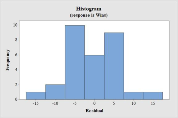
Assumption of normality from histogram:
- The majority of the observation in the middle and centered on the mean of 0.
- There are lower frequencies on the tails of the distributions.
According to the given histogram, the most of the observations are centered and there are fewer frequencies on the tails of the distributions. Thus, it can be considered as roughly symmetric.
Hence, the residuals follow a normal distribution.
h.
Plot the residual plot for the regression developed in Part (f).
h.
Explanation of Solution
Step by step procedure to obtain the residual Plot using MINITAB software:
- Choose Stat > Regression > Regression > Fit Regression Model.
- Under Responses, enter the column of Wins.
- Under Continuous predictors, enter the columns of BA and ERA.
- Choose Graphs.
- Under Residual plot select residual verses fits.
- Click OK.
The output obtained using Minitab is as follows:
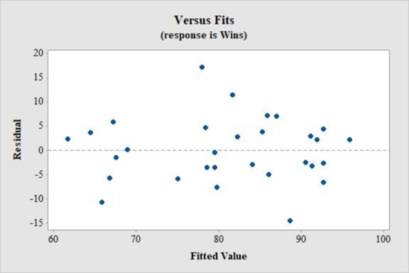
Assumption for residual analysis for the regression model:
- The plot of the residuals vs. the observed values of the predictor variable should fall roughly in a horizontal band and symmetric about x-axis.
- For a normal probability plot, residuals should be roughly linear.
- There should not be any observable pattern.
According to the given residual plot, the points are roughly scattered and moreover, there is no particular pattern in the residual plot. A complete haphazard and random nature has observed.
Want to see more full solutions like this?
Chapter 14 Solutions
Statistical Techniques in Business and Economics, 16th Edition


- Jensen Tire & Auto is deciding whether to purchase a maintenance contract for its newcomputer wheel alignment and balancing machine. Managers feel that maintenance expenseshould be related to usage, and they collected the following information on weeklyusage (hours) and annual maintenance expense (in hundreds of dollars). a. Develop a scatter chart with weekly usage hours as the independent variable. Whatdoes the scatter chart indicate about the relationship between weekly usage and annualmaintenance expense?b. Use the data to develop an estimated regression equation that could be used to predictthe annual maintenance expense for a given number of hours of weekly usage. Whatis the estimated regression model? c. Test whether each of the regression parameters b0 and b1 is equal to zero at a 0.05level of significance. What are the correct interpretations of the estimated regressionparameters? Are these interpretations reasonable?d. How much of the variation in the sample values of…arrow_forwardGiven the regression line Ý = 2.5X +12, what is the predicted value of self-esteem where X = 10arrow_forwardThe personnel director of a large hospital is interested in determining the relationship (if any) between an employee’s age and the number of sick days the employee takes per year. The director randomly selects ten employees and records their age and the number of sick days which they took in the previous year. Employee 1 2 3 4 5 6 7 8 9 10Age 30 50 40 55 30 28 60 25 30 45Sick Days 7 4 3 2 9 10 0 8 5 2 The estimated regression equation and the standard error are given. Sick Days=14.310162−0.236900(Age) Se=1.682207 Find the 95% prediction interval for the average number of sick days an employee will take per year, given the employee is 34 . Round your answer to two decimal places.arrow_forward
 Linear Algebra: A Modern IntroductionAlgebraISBN:9781285463247Author:David PoolePublisher:Cengage Learning
 Glencoe Algebra 1, Student Edition, 9780079039897...AlgebraISBN:9780079039897Author:CarterPublisher:McGraw Hill
 Big Ideas Math A Bridge To Success Algebra 1: Stu...AlgebraISBN:9781680331141Author:HOUGHTON MIFFLIN HARCOURTPublisher:Houghton Mifflin Harcourt