Chapter 17, Problem 9E

(a)

To determine

Sketch $y_3\left(t\right)$ and $y_5\left(t\right)$ for the periodic waveform $g\left(t\right)$ shown in Figure 17.29.

Answer to Problem 9E

The plot $y_3\left(t\right)$ and $y_5\left(t\right)$ for the periodic waveform $g\left(t\right)$ is sketched as shown in Figure 1.

Explanation of Solution

Given data:

Refer to Figure 17.29 in the textbook.

Formula used:

Write the general expression for Fourier series expansion.

$f\left(t\right)=a_0+{\displaystyle \sum _{n=1}^{\infty }\left(a_n\cos n{\omega }_{0}t+b_n\sin n{\omega }_{0}t\right)}$        (1)

Write the general expression for Fourier series coefficient $a_0$.

$a_0=\frac{1}{T}{\displaystyle {\int }_0^{T}f\left(t\right)}dt$        (2)

Write the general expression for Fourier series coefficient $a_n$.

$a_n=\frac{2}{T}{\displaystyle {\int }_0^{T}f\left(t\right)\cos n{\omega }_{0}t}dt$        (3)

Write the general expression for Fourier series coefficient $b_n$.

$b_n=\frac{2}{T}{\displaystyle {\int }_0^{T}f\left(t\right)\sin n{\omega }_{0}t}dt$        (4)

Write the expression to calculate the fundamental angular frequency.

${\omega }_0=\frac{2\pi }{T}=2\pi f_0$        (5)

Here,

$T$ is the period of the function.

Calculation:s

In the given Figure 17.29, the time period is $T=4$.

The function $v\left(t\right)$ for the given waveform is,

$g\left(t\right)=\{\begin{array}{l}-2t-4,t\le t-1\\ 2t,-1<t\le 1\\ -2t+4,1<t\le 3\end{array}$        (6)

Substitute 4 for T in equation (5) to find ${\omega }_0$.

${\omega }_0=\frac{2\pi }{4}$

${\omega }_0=\frac{\pi }{2}$        (7)

Applying equation (6) in equation (2) to find $a_0$ as follows,

$\begin{array}{c}{a}_0=\frac{1}{4}{\displaystyle {\int }_0^{4}f\left(t\right)}dt\\ =\frac{1}{4}\left[{\displaystyle {\int }_{-1}^1\left(2t\right)}dt+{\displaystyle {\int }_1^3\left(4-2t\right)}dt\right]\\ =\frac{1}{4}\left[2{\left[\frac{t^2}{2}\right]}_{-1}^1+{\left[4t-\frac{2t^2}{2}\right]}_1^3\right]\\ =\frac{1}{4}\left[2\left[\frac{{\left(1\right)}^2}{2}-\frac{{\left(1\right)}^2}{2}\right]-\left[\left(4\left(3\right)-\frac{2{\left(3\right)}^2}{2}\right)-\left(4\left(1\right)-\frac{2{\left(1\right)}^2}{2}\right)\right]\right]\end{array}$

Simplify the above equation as follows,

$\begin{array}{c}{a}_0=\frac{1}{4}\left[2\left[0\right]-\left[\left(12-9\right)-\left(4-1\right)\right]\right]\\ =\frac{1}{4}\left[0-\left(3-3\right)\right]\\ =0\end{array}$

Applying equation (6) in equation (3) to finding the Fourier coefficient $a_n$.

$a_n=\frac{2}{4}{\displaystyle {\int }_0^{4}f\left(t\right)\cos n{\omega }_{0}t}dt$

$a_n=\frac{1}{2}\left[{\displaystyle {\int }_{-1}^1\left(2t\right)\cos n{\omega }_{0}t}dt+{\displaystyle {\int }_1^3\left(4-2t\right)\cos n{\omega }_{0}t}dt\right]$        (8)

Equation (8) is simplified as,

$x={\displaystyle {\int }_{-1}^1\left(2t\right)\cos n{\omega }_{0}t}dt$

$y={\displaystyle {\int }_1^3\left(4-2t\right)\cos n{\omega }_{0}t}dt$

Therefore, equation (8) becomes,

$a_n=\frac{1}{2}\left[x+y\right]$        (9)

Consider the function,

$x=2{\displaystyle {\int }_{-1}^{1}t\cos n{\omega }_{0}t}dt$        (10)

Consider the following integration formula.

${\displaystyle \underset{a}{\overset{b}{\int }}udv}={\left[uv\right]}_a^b-{\displaystyle \underset{a}{\overset{b}{\int }}vdu}$        (11)

Compare the equations (10) and (11) to simplify the equation (10).

$\begin{array}{l}u=tdv=\cos n{\omega }_{0}tdt\\ du=dtv=\frac{\sin n{\omega }_{0}t}{n{\omega }_0}\end{array}$

Using the equation (11), the equation (10) can be reduced as,

$\begin{array}{c}x=2\left\{{\left[t\left(\frac{\sin n{\omega }_{0}t}{n{\omega }_0}\right)\right]}_{-1}^1-{\displaystyle {\int }_{-1}^1\left(\frac{\sin n{\omega }_{0}t}{n{\omega }_0}\right)dt}\right\}\\ =2\left\{\left[\left(1\right)\left(\frac{\sin n{\omega }_0\left(1\right)}{n{\omega }_0}\right)+\left(-1\right)\left(\frac{\sin n{\omega }_0\left(-1\right)}{n{\omega }_0}\right)\right]-{\left[\frac{-\cos n{\omega }_{0}t}{{\left(n{\omega }_0\right)}^2}\right]}_{-1}^1\right\}\\ =2\left\{\left[\left(\frac{\sin n{\omega }_0}{n{\omega }_0}\right)+\left(\frac{\sin n{\omega }_0}{n{\omega }_0}\right)\right]-\left[\frac{-\cos n{\omega }_0\left(1\right)}{{\left(n{\omega }_0\right)}^2}-\frac{-\cos n{\omega }_0\left(-1\right)}{{\left(n{\omega }_0\right)}^2}\right]\right\}\\ =2\left\{\left[\frac{2\sin n{\omega }_0}{n{\omega }_0}\right]-\left[\frac{-\cos n{\omega }_0}{{\left(n{\omega }_0\right)}^2}-\frac{\cos n{\omega }_0}{{\left(n{\omega }_0\right)}^2}\right]\right\}\end{array}$

Simplify the above equation as follows,

$\begin{array}{c}x=2\left\{\left[\frac{2\sin n{\omega }_0}{n{\omega }_0}\right]-\left[\frac{-2\cos n{\omega }_0}{{\left(n{\omega }_0\right)}^2}\right]\right\}\\ =\frac{4\sin n{\omega }_0}{n{\omega }_0}+\frac{4\cos n{\omega }_0}{{\left(n{\omega }_0\right)}^2}\end{array}$

Consider the function,

$y={\displaystyle {\int }_1^3\left(4-2t\right)\cos n{\omega }_{0}t}dt$        (12)

Compare the equations (12) and (11) to simplify the equation (12).

$\begin{array}{l}u=4-2tdv=\cos n{\omega }_{0}tdt\\ du=-2dtv=\frac{\sin n{\omega }_{0}t}{n{\omega }_0}\end{array}$

Using the equation (11), the equation (12) can be reduced as,

$\begin{array}{c}y={\left[\left(4-2t\right)\left(\frac{\sin n{\omega }_{0}t}{n{\omega }_0}\right)\right]}_1^3+2{\displaystyle {\int }_1^3\left(\frac{\sin n{\omega }_{0}t}{n{\omega }_0}\right)dt}\\ =\left[\left(4-2\left(3\right)\right)\left(\frac{\sin n{\omega }_0\left(3\right)}{n{\omega }_0}\right)-\left(4-2\left(1\right)\right)\left(\frac{\sin n{\omega }_0\left(1\right)}{n{\omega }_0}\right)\right]+2{\left[\frac{-\cos n{\omega }_{0}t}{{\left(n{\omega }_0\right)}^2}\right]}_1^3\\ =\left[\left(4-6\right)\left(\frac{\sin 3n{\omega }_0}{n{\omega }_0}\right)-\left(4-2\right)\left(\frac{\sin n{\omega }_0}{n{\omega }_0}\right)\right]+2\left[\frac{-\cos n{\omega }_0\left(3\right)}{{\left(n{\omega }_0\right)}^2}-\frac{-\cos n{\omega }_0\left(1\right)}{{\left(n{\omega }_0\right)}^2}\right]\\ =\left[\left(-2\right)\left(\frac{\sin 3n{\omega }_0}{n{\omega }_0}\right)-\left(2\right)\left(\frac{\sin n{\omega }_0}{n{\omega }_0}\right)\right]+2\left[\frac{-\cos 3n{\omega }_0}{{\left(n{\omega }_0\right)}^2}+\frac{\cos n{\omega }_0}{{\left(n{\omega }_0\right)}^2}\right]\\ =-\frac{2\sin 3n{\omega }_0}{n{\omega }_0}-\frac{2\sin n{\omega }_0}{n{\omega }_0}-\frac{2\cos 3n{\omega }_0}{{\left(n{\omega }_0\right)}^2}+\frac{2\cos n{\omega }_0}{{\left(n{\omega }_0\right)}^2}\end{array}$

Substitute the value of x and y in equation (9) as follows,

$\begin{array}{c}{a}_n=\frac{1}{2}\left[\frac{4\sin n{\omega }_0}{n{\omega }_0}+\frac{4\cos n{\omega }_0}{{\left(n{\omega }_0\right)}^2}-\frac{2\sin 3n{\omega }_0}{n{\omega }_0}-\frac{2\sin n{\omega }_0}{n{\omega }_0}-\frac{2\cos 3n{\omega }_0}{{\left(n{\omega }_0\right)}^2}+\frac{2\cos n{\omega }_0}{{\left(n{\omega }_0\right)}^2}\right]\\ =\frac{2\sin n{\omega }_0}{n{\omega }_0}+\frac{2\cos n{\omega }_0}{{\left(n{\omega }_0\right)}^2}-\frac{\sin 3n{\omega }_0}{n{\omega }_0}-\frac{\sin n{\omega }_0}{n{\omega }_0}-\frac{\cos 3n{\omega }_0}{{\left(n{\omega }_0\right)}^2}+\frac{\cos n{\omega }_0}{{\left(n{\omega }_0\right)}^2}\\ =\frac{2\sin n\left(\frac{\pi }{2}\right)}{n\left(\frac{\pi }{2}\right)}+\frac{2\cos n\left(\frac{\pi }{2}\right)}{{\left(n\left(\frac{\pi }{2}\right)\right)}^2}-\frac{\sin 3n\left(\frac{\pi }{2}\right)}{n\left(\frac{\pi }{2}\right)}-\frac{\sin n\left(\frac{\pi }{2}\right)}{n\left(\frac{\pi }{2}\right)}-\frac{\cos 3n\left(\frac{\pi }{2}\right)}{{\left(n\left(\frac{\pi }{2}\right)\right)}^2}+\frac{\cos n\left(\frac{\pi }{2}\right)}{{\left(n\left(\frac{\pi }{2}\right)\right)}^2}\\ \left\{\because {\omega }_0=\frac{\pi }{2}\right\}\\ =\frac{\sin n\pi }{\frac{n\pi }{2}}+\frac{\cos n\pi }{{\left(\frac{n\pi }{2}\right)}^2}-\frac{\sin 3n\left(\frac{\pi }{2}\right)}{\frac{n\pi }{2}}-\frac{\sin n\left(\frac{\pi }{2}\right)}{\frac{n\pi }{2}}-\frac{\cos 3n\left(\frac{\pi }{2}\right)}{{\left(\frac{n\pi }{2}\right)}^2}+\frac{\cos n\left(\frac{\pi }{2}\right)}{{\left(\frac{n\pi }{2}\right)}^2}\end{array}$

The above equation becomes,

$a_n=\frac{2\sin n\pi }{n\pi }+\frac{4\cos n\pi }{{\left(n\pi \right)}^2}-\frac{2\sin 3n\left(\frac{\pi }{2}\right)}{n\pi }-\frac{2\sin n\left(\frac{\pi }{2}\right)}{n\pi }-\frac{4\cos 3n\left(\frac{\pi }{2}\right)}{{\left(n\pi \right)}^2}+\frac{4\cos n\left(\frac{\pi }{2}\right)}{{\left(n\pi \right)}^2}$$a_n=\frac{2\sin n\pi }{n\pi }+\frac{4\cos n\pi }{{\left(n\pi \right)}^2}-\frac{\sin 3n\pi }{n\pi }-\frac{\sin n\pi }{n\pi }-\frac{2\cos 3n\pi }{{\left(n\pi \right)}^2}+\frac{2\cos n\pi }{{\left(n\pi \right)}^2}$        (13)

Applying equation (6) in equation (4) to finding the Fourier coefficient $b_n$.

$b_n=\frac{2}{4}{\displaystyle {\int }_0^{4}f\left(t\right)\sin n{\omega }_{0}t}dt$

$b_n=\frac{1}{2}\left[{\displaystyle {\int }_{-1}^1\left(2t\right)\sin n{\omega }_{0}t}dt+{\displaystyle {\int }_1^3\left(4-2t\right)\sin n{\omega }_{0}t}dt\right]$        (14)

Equation (14) is simplified as,

$m={\displaystyle {\int }_{-1}^1\left(2t\right)\sin n{\omega }_{0}t}dt$

$n={\displaystyle {\int }_1^3\left(4-2t\right)\sin n{\omega }_{0}t}dt$

Therefore, equation (14) becomes,

$b_n=\frac{1}{2}\left[m+n\right]$        (15)

Consider the function,

$m=2{\displaystyle {\int }_{-1}^{1}t\sin n{\omega }_{0}t}dt$        (16)

Consider the following integration formula.

${\displaystyle \underset{a}{\overset{b}{\int }}udv}={\left[uv\right]}_a^b-{\displaystyle \underset{a}{\overset{b}{\int }}vdu}$        (17)

Compare the equations (17) and (16) to simplify the equation (16).

$\begin{array}{l}u=tdv=\sin n{\omega }_{0}td\\ du=dtv=\frac{-\cos n{\omega }_{0}t}{n{\omega }_0}\end{array}$

Using the equation (17), the equation (16) can be reduced as,

$\begin{array}{c}m=2\left\{{\left[t\left(\frac{-\cos n{\omega }_{0}t}{n{\omega }_0}\right)\right]}_{-1}^1-{\displaystyle {\int }_{-1}^1\left(\frac{-\cos n{\omega }_{0}t}{n{\omega }_0}\right)dt}\right\}\\ =2\left\{\left[\left(1\right)\left(\frac{-\cos n{\omega }_0\left(1\right)}{n{\omega }_0}\right)-\left(-1\right)\left(\frac{-\cos n{\omega }_0\left(-1\right)}{n{\omega }_0}\right)\right]-{\left[\frac{-\sin n{\omega }_{0}t}{{\left(n{\omega }_0\right)}^2}\right]}_{-1}^1\right\}\\ =2\left\{\left[\left(\frac{-\cos n{\omega }_0}{n{\omega }_0}\right)+\left(\frac{\cos n{\omega }_0}{n{\omega }_0}\right)\right]-\left[\frac{-\sin n{\omega }_0\left(1\right)}{{\left(n{\omega }_0\right)}^2}-\frac{-\sin n{\omega }_0\left(-1\right)}{{\left(n{\omega }_0\right)}^2}\right]\right\}\\ =\left[\frac{-2\cos n{\omega }_0}{n{\omega }_0}+\frac{2\cos n{\omega }_0}{n{\omega }_0}\right]-\left[\frac{-2\sin n{\omega }_0}{{\left(n{\omega }_0\right)}^2}-\frac{2\sin n{\omega }_0}{{\left(n{\omega }_0\right)}^2}\right]\end{array}$

Simplify the above equation as follows,

$\begin{array}{c}m=\frac{-2\cos n{\omega }_0}{n{\omega }_0}+\frac{2\cos n{\omega }_0}{n{\omega }_0}+\frac{2\sin n{\omega }_0}{{\left(n{\omega }_0\right)}^2}+\frac{2\sin n{\omega }_0}{{\left(n{\omega }_0\right)}^2}\\ =\frac{4\sin n{\omega }_0}{{\left(n{\omega }_0\right)}^2}\end{array}$

Consider the function,

$n={\displaystyle {\int }_1^3\left(4-2t\right)\sin n{\omega }_{0}t}dt$        (18)

Compare the equations (17) and (18) to simplify the equation (18).

$\begin{array}{l}u=4-2tdv=\sin n{\omega }_{0}tdt\\ du=-2dtv=\frac{-\cos n{\omega }_{0}t}{n{\omega }_0}\end{array}$

Using the equation (17), the equation (18) can be reduced as,

$\begin{array}{c}n={\left[\left(4-2t\right)\left(\frac{-\cos n{\omega }_{0}t}{n{\omega }_0}\right)\right]}_1^3-2{\displaystyle {\int }_1^3\left(\frac{\cos n{\omega }_{0}t}{n{\omega }_0}\right)dt}\\ =\left[\left(4-2\left(3\right)\right)\left(\frac{-\cos n{\omega }_0\left(3\right)}{n{\omega }_0}\right)-\left(4-2\left(1\right)\right)\left(\frac{-\cos n{\omega }_0\left(1\right)}{n{\omega }_0}\right)\right]-2{\left[\frac{\sin n{\omega }_{0}t}{{\left(n{\omega }_0\right)}^2}\right]}_1^3\\ =\left[\left(-2\right)\left(\frac{-\cos 3n{\omega }_0}{n{\omega }_0}\right)-\left(2\right)\left(\frac{-\cos n{\omega }_0}{n{\omega }_0}\right)\right]-2\left[\frac{\sin n{\omega }_0\left(3\right)}{{\left(n{\omega }_0\right)}^2}-\frac{\sin n{\omega }_0\left(1\right)}{{\left(n{\omega }_0\right)}^2}\right]\\ =\left[\left(\frac{2\cos 3n{\omega }_0}{n{\omega }_0}\right)+\left(\frac{2\cos n{\omega }_0}{n{\omega }_0}\right)\right]-2\left[\frac{\sin 3n{\omega }_0}{{\left(n{\omega }_0\right)}^2}-\frac{\sin n{\omega }_0}{{\left(n{\omega }_0\right)}^2}\right]\\ =\frac{2\cos 3n{\omega }_0}{n{\omega }_0}+\frac{2\cos n{\omega }_0}{n{\omega }_0}-\frac{2\sin 3n{\omega }_0}{{\left(n{\omega }_0\right)}^2}+\frac{2\sin n{\omega }_0}{{\left(n{\omega }_0\right)}^2}\end{array}$

Substitute the values of m and n in equation (15) as follows,

$\begin{array}{c}{b}_n=\frac{1}{2}\left[\frac{4\sin n{\omega }_0}{{\left(n{\omega }_0\right)}^2}+\frac{2\cos 3n{\omega }_0}{n{\omega }_0}+\frac{2\cos n{\omega }_0}{n{\omega }_0}-\frac{2\sin 3n{\omega }_0}{{\left(n{\omega }_0\right)}^2}+\frac{2\sin n{\omega }_0}{{\left(n{\omega }_0\right)}^2}\right]\\ =\frac{1}{2}\left[\frac{4\sin n\left(\frac{\pi }{2}\right)}{{\left(n\left(\frac{\pi }{2}\right)\right)}^2}+\frac{2\cos 3n\left(\frac{\pi }{2}\right)}{n\left(\frac{\pi }{2}\right)}+\frac{2\cos n\left(\frac{\pi }{2}\right)}{n\left(\frac{\pi }{2}\right)}-\frac{2\sin 3n\left(\frac{\pi }{2}\right)}{{\left(n\left(\frac{\pi }{2}\right)\right)}^2}+\frac{2\sin n\left(\frac{\pi }{2}\right)}{{\left(n\left(\frac{\pi }{2}\right)\right)}^2}\right]\\ =\frac{1}{2}\left[\frac{2\sin n\pi }{{\left(n\left(\frac{\pi }{2}\right)\right)}^2}+\frac{\cos 3n\pi }{n\left(\frac{\pi }{2}\right)}+\frac{\cos n\pi }{n\left(\frac{\pi }{2}\right)}-\frac{\sin 3n\pi }{{\left(n\left(\frac{\pi }{2}\right)\right)}^2}+\frac{\sin n\pi }{{\left(n\left(\frac{\pi }{2}\right)\right)}^2}\right]\\ =\frac{\sin n\pi }{\frac{{\left(n\pi \right)}^2}{4}}+\frac{\cos 3n\pi }{n\pi }+\frac{\cos n\pi }{n\pi }-\frac{\sin 3n\pi }{\frac{{\left(n\pi \right)}^2}{2}}+\frac{\sin n\pi }{\frac{{\left(n\pi \right)}^2}{2}}\end{array}$

The above equation becomes,

$b_n=\frac{2\sin n\pi }{{\left(n\pi \right)}^2}+\frac{\cos 3n\pi }{n\pi }+\frac{\cos n\pi }{n\pi }-\frac{2\sin 3n\pi }{{\left(n\pi \right)}^2}+\frac{2\sin n\pi }{{\left(n\pi \right)}^2}$

Substitute the values of $a_0$, $a_n$, and $b_n$ in equation (1) as follows,

$\begin{array}{c}g\left(t\right)=0+{\displaystyle \sum _{n=1}^{\infty }\left[\left(\begin{array}{l}\frac{2\sin n\pi }{n\pi }+\frac{4\cos n\pi }{{\left(n\pi \right)}^2}-\frac{\sin 3n\pi }{n\pi }\\ -\frac{\sin n\pi }{n\pi }-\frac{2\cos 3n\pi }{{\left(n\pi \right)}^2}+\frac{2\cos n\pi }{{\left(n\pi \right)}^2}\end{array}\right)\cos n\left(\frac{\pi }{2}\right)t\right]}\\ +{\displaystyle \sum _{n=1}^{\infty }\left[\left(\begin{array}{l}\frac{2\sin n\pi }{{\left(n\pi \right)}^2}+\frac{\cos 3n\pi }{n\pi }+\frac{\cos n\pi }{n\pi }\\ -\frac{2\sin 3n\pi }{{\left(n\pi \right)}^2}+\frac{2\sin n\pi }{{\left(n\pi \right)}^2}\end{array}\right)\cos n\left(\frac{\pi }{2}\right)t\right]}\\ ={\displaystyle \sum _{n=1}^{\infty }\left[\left(\begin{array}{l}0+\frac{4{\left(-1\right)}^n}{{\left(n\pi \right)}^2}-0\\ -0-\frac{2\cos 3n\pi }{{\left(n\pi \right)}^2}+\frac{2{\left(-1\right)}^n}{{\left(n\pi \right)}^2}\end{array}\right)\cos n\left(\frac{\pi }{2}\right)t\right]}\\ +{\displaystyle \sum _{n=1}^{\infty }\left[\left(\begin{array}{l}0+\frac{\cos 3n\pi }{n\pi }+\frac{{\left(-1\right)}^n}{n\pi }\\ -0+0\end{array}\right)\cos n\left(\frac{\pi }{2}\right)t\right]}\\ ={\displaystyle \sum _{n=1}^{\infty }\left[\left(\frac{4{\left(-1\right)}^n}{{\left(n\pi \right)}^2}-\frac{2\cos 3n\pi }{{\left(n\pi \right)}^2}+\frac{2{\left(-1\right)}^n}{{\left(n\pi \right)}^2}\right)\cos n\left(\frac{\pi }{2}\right)t\right]}\\ +{\displaystyle \sum _{n=1}^{\infty }\left[\left(\frac{\cos 3n\pi }{n\pi }+\frac{{\left(-1\right)}^n}{n\pi }\right)\cos n\left(\frac{\pi }{2}\right)t\right]}\end{array}$        (19)

$g\left(t\right)={\displaystyle \sum _{n=1}^{\infty }\left[\left(\frac{6{\left(-1\right)}^n}{{\left(n\pi \right)}^2}-\frac{2\cos 3n\pi }{{\left(n\pi \right)}^2}\right)\cos n\left(\frac{\pi }{2}\right)t\right]}+{\displaystyle \sum _{n=1}^{\infty }\left[\left(\frac{\cos 3n\pi }{n\pi }+\frac{{\left(-1\right)}^n}{n\pi }\right)\cos n\left(\frac{\pi }{2}\right)t\right]}$

The above equation becomes,

$g\left(t\right)={\displaystyle \sum _{n=1}^{\infty }\left[\left(\frac{6{\left(-1\right)}^n-2\cos 3n\pi }{{\left(n\pi \right)}^2}\right)\cos n\left(\frac{\pi }{2}\right)t\right]}+{\displaystyle \sum _{n=1}^{\infty }\left[\left(\frac{\cos 3n\pi +{\left(-1\right)}^n}{n\pi }\right)\cos n\left(\frac{\pi }{2}\right)t\right]}$

For $n=1$,

$y_1\left(t\right)=g\left(t\right)$ have the Fourier coefficients $a_o$, $a_1$ and $b_1$.

Therefore, equation (19) will be as follows,

$\begin{array}{c}{y}_1\left(t\right)=\left[\left(\frac{2\sin \pi }{\pi }+\frac{4\cos \pi }{{\left(\pi \right)}^2}-\frac{\sin \pi }{\pi }-\frac{\sin \pi }{\pi }-\frac{2\cos 3\pi }{{\left(\pi \right)}^2}+\frac{2\cos \pi }{{\left(\pi \right)}^2}\right)\cos \left(\frac{\pi }{2}\right)t\right]+\\ \left[\left(\frac{2\sin \pi }{{\left(3\pi \right)}^2}+\frac{\cos 3\pi }{3\pi }+\frac{\cos \pi }{3\pi }-\frac{2\sin 3\pi }{{\left(3\pi \right)}^2}+\frac{2\sin \pi }{{\left(3\pi \right)}^2}\right)\cos \left(\frac{\pi }{2}\right)t\right]+\\ =\left[\left(0-\frac{4}{{\left(\pi \right)}^2}-0-0+\frac{2}{{\left(\pi \right)}^2}-\frac{2}{{\left(\pi \right)}^2}\right)\cos \left(\frac{\pi }{2}\right)t\right]+\left[\left(0-\frac{1}{3\pi }-\frac{1}{3\pi }+0+0\right)\cos \left(\frac{\pi }{2}\right)t\right]\end{array}$

$y_1\left(t\right)=\left[\frac{4}{{\pi }^2}\cos \left(\frac{\pi }{2}\right)t\right]-\left[\frac{2}{3\pi }\cos \left(\frac{\pi }{2}\right)t\right]$

For $n=2$,

$y_2\left(t\right)=g\left(t\right)$ have the Fourier coefficients $a_o$, $a_1$, $a_2$ and $b_1$, $b_2$.

Therefore, equation (19) will be as follows,

$\begin{array}{c}{y}_2\left(t\right)=\left[\left(\frac{2\sin \pi }{\pi }+\frac{4\cos \pi }{{\left(\pi \right)}^2}-\frac{\sin \pi }{\pi }-\frac{\sin \pi }{\pi }-\frac{2\cos 3\pi }{{\left(\pi \right)}^2}+\frac{2\cos \pi }{{\left(\pi \right)}^2}\right)\cos \left(\frac{\pi }{2}\right)t\right]+\\ \left[\left(\frac{2\sin \pi }{{\left(3\pi \right)}^2}+\frac{\cos 3\pi }{3\pi }+\frac{\cos \pi }{3\pi }-\frac{2\sin 3\pi }{{\left(3\pi \right)}^2}+\frac{2\sin \pi }{{\left(3\pi \right)}^2}\right)\cos \left(\frac{\pi }{2}\right)t\right]+\\ \left[\left(\frac{2\sin 2\pi }{2\pi }+\frac{4\cos 2\pi }{{\left(2\pi \right)}^2}-\frac{\sin 6\pi }{2\pi }-\frac{\sin 2\pi }{2\pi }-\frac{2\cos 6\pi }{{\left(2\pi \right)}^2}+\frac{2\cos 2\pi }{{\left(2\pi \right)}^2}\right)\cos 2\left(\frac{\pi }{2}\right)t\right]+\\ \left[\left(\frac{2\sin 2\pi }{{\left(2\pi \right)}^2}+\frac{\cos 6\pi }{2\pi }+\frac{\cos 2\pi }{2\pi }-\frac{2\sin 6\pi }{{\left(2\pi \right)}^2}+\frac{2\sin 2\pi }{{\left(2\pi \right)}^2}\right)\cos 2\left(\frac{\pi }{2}\right)t\right]+\\ =\left[\left(0-\frac{4}{{\left(\pi \right)}^2}-0-0+\frac{2}{{\left(\pi \right)}^2}-\frac{2}{{\left(\pi \right)}^2}\right)\cos \left(\frac{\pi }{2}\right)t\right]+\left[\left(0-\frac{1}{3\pi }-\frac{1}{3\pi }+0+0\right)\cos \left(\frac{\pi }{2}\right)t\right]+\\ \left[\left(0+\frac{4}{{\left(2\pi \right)}^2}-0-0-\frac{2}{{\left(2\pi \right)}^2}+\frac{2}{{\left(2\pi \right)}^2}\right)\cos 2\left(\frac{\pi }{2}\right)t\right]+\left[\left(0+\frac{1}{2\pi }+\frac{1}{2\pi }-0+0\right)\cos 2\left(\frac{\pi }{2}\right)t\right]\end{array}$$y_2\left(t\right)=\left[\frac{4}{{\pi }^2}\cos \left(\frac{\pi }{2}\right)t\right]-\left[\frac{2}{3\pi }\cos \left(\frac{\pi }{2}\right)t\right]+\left[\frac{1}{{\pi }^2}\cos 2\left(\frac{\pi }{2}\right)t\right]+\left[\frac{1}{\pi }\cos 2\left(\frac{\pi }{2}\right)t\right]$

For $n=3$,

$y_3\left(t\right)=g\left(t\right)$ have the Fourier coefficients $a_o$, $a_1$, $a_2$, $a_3$ and $b_1$, $b_2$, $b_3$.

Therefore, equation (19) will be as follows,

$\begin{array}{l}{y}_3\left(t\right)=\left[\left(\frac{2\sin \pi }{\pi }+\frac{4\cos \pi }{{\left(\pi \right)}^2}-\frac{\sin \pi }{\pi }-\frac{\sin \pi }{\pi }-\frac{2\cos 3\pi }{{\left(\pi \right)}^2}+\frac{2\cos \pi }{{\left(\pi \right)}^2}\right)\cos \left(\frac{\pi }{2}\right)t\right]+\\ \left[\left(\frac{2\sin \pi }{{\left(3\pi \right)}^2}+\frac{\cos 3\pi }{3\pi }+\frac{\cos \pi }{3\pi }-\frac{2\sin 3\pi }{{\left(3\pi \right)}^2}+\frac{2\sin \pi }{{\left(3\pi \right)}^2}\right)\cos \left(\frac{\pi }{2}\right)t\right]+\\ \left[\left(\frac{2\sin 2\pi }{2\pi }+\frac{4\cos 2\pi }{{\left(2\pi \right)}^2}-\frac{\sin 6\pi }{2\pi }-\frac{\sin 2\pi }{2\pi }-\frac{2\cos 6\pi }{{\left(2\pi \right)}^2}+\frac{2\cos 2\pi }{{\left(2\pi \right)}^2}\right)\cos 2\left(\frac{\pi }{2}\right)t\right]+\\ \left[\left(\frac{2\sin 2\pi }{{\left(2\pi \right)}^2}+\frac{\cos 6\pi }{2\pi }+\frac{\cos 2\pi }{2\pi }-\frac{2\sin 6\pi }{{\left(2\pi \right)}^2}+\frac{2\sin 2\pi }{{\left(2\pi \right)}^2}\right)\cos 2\left(\frac{\pi }{2}\right)t\right]+\\ \left[\left(\frac{2\sin 3\pi }{3\pi }+\frac{4\cos 3\pi }{{\left(3\pi \right)}^2}-\frac{\sin 9\pi }{3\pi }-\frac{\sin 3\pi }{3\pi }-\frac{2\cos 9\pi }{{\left(3\pi \right)}^2}+\frac{2\cos 3\pi }{{\left(3\pi \right)}^2}\right)\cos 3\left(\frac{\pi }{2}\right)t\right]+\\ \left[\left(\frac{2\sin 3\pi }{{\left(3\pi \right)}^2}+\frac{\cos 9\pi }{3\pi }+\frac{\cos 3\pi }{3\pi }-\frac{2\sin 9\pi }{{\left(3\pi \right)}^2}+\frac{2\sin 3\pi }{{\left(3\pi \right)}^2}\right)\cos 3\left(\frac{\pi }{2}\right)t\right]\end{array}$

$\begin{array}{c}{y}_3\left(t\right)=\left[\left(0-\frac{4}{{\left(\pi \right)}^2}-0-0+\frac{2}{{\left(\pi \right)}^2}-\frac{2}{{\left(\pi \right)}^2}\right)\cos \left(\frac{\pi }{2}\right)t\right]+\left[\left(0-\frac{1}{3\pi }-\frac{1}{3\pi }+0+0\right)\cos \left(\frac{\pi }{2}\right)t\right]+\\ \left[\left(0+\frac{4}{{\left(2\pi \right)}^2}-0-0-\frac{2}{{\left(2\pi \right)}^2}+\frac{2}{{\left(2\pi \right)}^2}\right)\cos 2\left(\frac{\pi }{2}\right)t\right]+\left[\left(0+\frac{1}{2\pi }+\frac{1}{2\pi }-0+0\right)\cos 2\left(\frac{\pi }{2}\right)t\right]\\ +\left[\left(0-\frac{4}{{\left(3\pi \right)}^2}-0-0+\frac{2}{{\left(3\pi \right)}^2}-\frac{2}{{\left(3\pi \right)}^2}\right)\cos 3\left(\frac{\pi }{2}\right)t\right]\\ +\left[\left(0-\frac{1}{3\pi }-\frac{1}{3\pi }-0+0\right)\cos 3\left(\frac{\pi }{2}\right)t\right]\\ =\left[\frac{4}{{\pi }^2}\cos \left(\frac{\pi }{2}\right)t\right]-\left[\frac{2}{3\pi }\cos \left(\frac{\pi }{2}\right)t\right]+\left[\frac{1}{{\pi }^2}\cos 2\left(\frac{\pi }{2}\right)t\right]+\left[\frac{1}{\pi }\cos 2\left(\frac{\pi }{2}\right)t\right]\\ +\left[\frac{4}{9{\pi }^2}\cos 3\left(\frac{\pi }{2}\right)t\right]-\left[\frac{2}{3\pi }\cos 3\left(\frac{\pi }{2}\right)t\right]\\ =\left[\frac{4}{{\pi }^2}-\frac{2}{3\pi }\right]\cos \left(\frac{\pi }{2}\right)t+\left[\frac{1}{{\pi }^2}+\frac{1}{\pi }\right]\cos 2\left(\frac{\pi }{2}\right)t+\left[\frac{4}{9{\pi }^2}-\frac{2}{3\pi }\right]\cos 3\left(\frac{\pi }{2}\right)t\\ =0.193\cos \left(\frac{\pi }{2}\right)t+0.419\cos 2\left(\frac{\pi }{2}\right)t-0.167\cos 3\left(\frac{\pi }{2}\right)t\end{array}$

Similarly, for $n=5$,

$y_5\left(t\right)=g\left(t\right)$ have the Fourier coefficients $a_o$, $a_1$, $a_2$, $a_3$, $a_4$, $a_5$ and $b_1$, $b_2$, $b_3$, $b_4$, $b_5$.

Therefore, equation (19) will be as follows,

$\begin{array}{c}{y}_5\left(t\right)=y_3\left(t\right)+\left[\left(\begin{array}{l}\frac{2\sin 4\pi }{4\pi }+\frac{4\cos 4\pi }{{\left(4\pi \right)}^2}-\frac{\sin 12\pi }{4\pi }\\ -\frac{\sin 4\pi }{4\pi }-\frac{2\cos 12\pi }{{\left(4\pi \right)}^2}+\frac{2\cos 4\pi }{{\left(4\pi \right)}^2}\end{array}\right)\cos 4\left(\frac{\pi }{2}\right)t\right]\\ +\left[\left(\begin{array}{l}\frac{2\sin 4\pi }{{\left(4\pi \right)}^2}+\frac{\cos 12\pi }{4\pi }+\frac{\cos 4\pi }{4\pi }\\ -\frac{2\sin 12\pi }{{\left(4\pi \right)}^2}+\frac{2\sin 4\pi }{{\left(4\pi \right)}^2}\end{array}\right)\cos 4\left(\frac{\pi }{2}\right)t\right]\\ +\left[\left(\begin{array}{l}\frac{2\sin 5\pi }{5\pi }+\frac{4\cos 5\pi }{{\left(5\pi \right)}^2}-\frac{\sin 15\pi }{5\pi }\\ -\frac{\sin 5\pi }{5\pi }-\frac{2\cos 15\pi }{{\left(5\pi \right)}^2}+\frac{2\cos 5\pi }{{\left(5\pi \right)}^2}\end{array}\right)\cos 5\left(\frac{\pi }{2}\right)t\right]\\ +\left[\left(\begin{array}{l}\frac{2\sin 5\pi }{{\left(5\pi \right)}^2}+\frac{\cos 15\pi }{5\pi }+\frac{\cos 5\pi }{5\pi }\\ -\frac{2\sin 15\pi }{{\left(5\pi \right)}^2}+\frac{2\sin 5\pi }{{\left(5\pi \right)}^2}\end{array}\right)\cos 5\left(\frac{\pi }{2}\right)t\right]\\ =\left[\frac{4}{{\pi }^2}\cos \left(\frac{\pi }{2}\right)t\right]-\left[\frac{2}{3\pi }\cos \left(\frac{\pi }{2}\right)t\right]+\left[\frac{1}{{\pi }^2}\cos 2\left(\frac{\pi }{2}\right)t\right]\\ +\left[\frac{1}{\pi }\cos 2\left(\frac{\pi }{2}\right)t\right]+\left[\frac{4}{9{\pi }^2}\cos 3\left(\frac{\pi }{2}\right)t\right]-\left[\frac{2}{3\pi }\cos 3\left(\frac{\pi }{2}\right)t\right]\\ +\left[\left(0+\frac{4}{{\left(4\pi \right)}^2}-0-0-\frac{2}{{\left(4\pi \right)}^2}+\frac{2}{{\left(4\pi \right)}^2}\right)\cos 4\left(\frac{\pi }{2}\right)t\right]\\ +\left[\left(0+\frac{1}{4\pi }+\frac{1}{4\pi }-0+0\right)\cos 4\left(\frac{\pi }{2}\right)t\right]\\ +\left[\left(0-\frac{4}{{\left(5\pi \right)}^2}-0-0+\frac{2}{{\left(5\pi \right)}^2}-\frac{2}{{\left(5\pi \right)}^2}\right)\cos 5\left(\frac{\pi }{2}\right)t\right]\\ +\left[\left(0-\frac{1}{5\pi }-\frac{1}{5\pi }-0+0\right)\cos 5\left(\frac{\pi }{2}\right)t\right]\end{array}$

$\begin{array}{c}{y}_5\left(t\right)=\left[\frac{4}{{\pi }^2}\cos \left(\frac{\pi }{2}\right)t\right]-\left[\frac{2}{3\pi }\cos \left(\frac{\pi }{2}\right)t\right]+\left[\frac{1}{{\pi }^2}\cos 2\left(\frac{\pi }{2}\right)t\right]\\ +\left[\frac{1}{\pi }\cos 2\left(\frac{\pi }{2}\right)t\right]+\left[\frac{4}{9{\pi }^2}\cos 3\left(\frac{\pi }{2}\right)t\right]-\left[\frac{2}{3\pi }\cos 3\left(\frac{\pi }{2}\right)t\right]\\ +\left[\frac{1}{4{\pi }^2}\cos 4\left(\frac{\pi }{2}\right)t\right]+\left[\frac{1}{2\pi }\cos 4\left(\frac{\pi }{2}\right)t\right]-\left[\frac{4}{25{\pi }^2}\cos 5\left(\frac{\pi }{2}\right)t\right]-\left[\frac{2}{5\pi }\cos 5\left(\frac{\pi }{2}\right)t\right]\\ =\left[\frac{4}{{\pi }^2}-\frac{2}{3\pi }\right]\cos \left(\frac{\pi }{2}\right)t+\left[\frac{1}{{\pi }^2}+\frac{1}{\pi }\right]\cos 2\left(\frac{\pi }{2}\right)t+\left[\frac{4}{9{\pi }^2}-\frac{2}{3\pi }\right]\cos 3\left(\frac{\pi }{2}\right)t\\ +\left[\frac{1}{4{\pi }^2}+\frac{1}{2\pi }\right]\cos 4\left(\frac{\pi }{2}\right)t-\left[\frac{4}{25{\pi }^2}+\frac{2}{5\pi }\right]\cos 5\left(\frac{\pi }{2}\right)t\\ y_5\left(t\right)=0.193\cos \left(\frac{\pi }{2}\right)t+0.419\cos 2\left(\frac{\pi }{2}\right)t-0.167\cos 3\left(\frac{\pi }{2}\right)t\\ +0.184\cos 4\left(\frac{\pi }{2}\right)t-0.143\cos 5\left(\frac{\pi }{2}\right)t\end{array}$

Write the MATLAB Code to plot $y_3\left(t\right)$, $y_5\left(t\right)$ along with $g\left(t\right)$ as follows:

t=linspace(-3,5,1000);

g0=0;

N=40;

for i=1:1000;

   y3=0.193*cos(pi*t/2) + 0.419*cos(pi*t) - 0.167*cos(3*pi*t/2);

   y5=0.193*cos(pi*t/2) + 0.419*cos(pi*t) - 0.167*cos(3*pi*t/2) + 0.184*cos(2*pi*t) - 0.143*cos(5*pi*t/2);

end

for i=1:1000;

sum=0;  

    for n=1:N;     

      sum=sum+((6*(-1)^n - 2*cos(3*n*pi))/(n*pi)^2)*cos(n*pi*t(i)/2) +  (((-1)^n + cos(3*n*pi))/(n*pi))*cos(n*pi*t(i)/2);

    end

gt(i)=g0+sum;

end

plot(t,y3,'b', t,y5,'r', t,gt,'g')

legend({'y3','y5','gt'},'Location','best')

xlabel('Time t in sec')

ylabel('The values y3, y5, and gt')

title('Plots for y3, y5, and gt')

Matlab output:

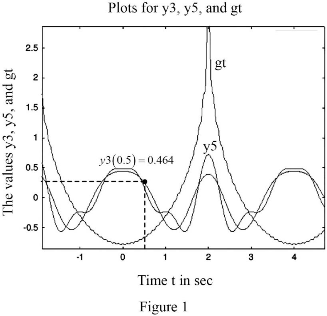
Figure 1 shows the plot $y_3\left(t\right)$, $y_5\left(t\right)$ along with $g\left(t\right)$.

Conclusion:

Thus, the plot $y_3\left(t\right)$ and $y_5\left(t\right)$ for the periodic waveform $g\left(t\right)$ is sketched as shown in Figure 1.

(b)

To determine

Find the values of $y_1\left(0.5\right)$, $y_2\left(0.5\right)$, $y_3\left(0.5\right)$, and $g\left(0.5\right)$

Answer to Problem 9E

The values of $y_1\left(0.5\right)$, $y_2\left(0.5\right)$, $y_3\left(0.5\right)$, and $g\left(0.5\right)$ is determined.

Explanation of Solution

Given data:

Refer to Figure 17.29 in the textbook.

Calculation:

From Part (a), the function $g\left(t\right)$ is,

$g\left(t\right)={\displaystyle \sum _{n=1}^{\infty }\left[\left(\frac{6{\left(-1\right)}^n-2\cos 3n\pi }{{\left(n\pi \right)}^2}\right)\cos n\left(\frac{\pi }{2}\right)t\right]}+{\displaystyle \sum _{n=1}^{\infty }\left[\left(\frac{\cos 3n\pi +{\left(-1\right)}^n}{n\pi }\right)\cos n\left(\frac{\pi }{2}\right)t\right]}$

Finding $g\left(0.5\right)$,

$\begin{array}{c}g\left(0.5\right)=\left[\left(\frac{6{\left(-1\right)}^{\left(1\right)}-2\cos 3\left(1\right)\pi }{{\left(\left(1\right)\pi \right)}^2}\right)\cos 0.5\left(1\right)\left(\frac{\pi }{2}\right)\right]+\left[\left(\frac{\cos 3\left(1\right)\pi +{\left(-1\right)}^{\left(1\right)}}{\left(1\right)\pi }\right)\cos 0.5\left(1\right)\left(\frac{\pi }{2}\right)\right]\\ +\left[\left(\frac{6{\left(-1\right)}^{\left(2\right)}-2\cos 3\left(2\right)\pi }{{\left(\left(2\right)\pi \right)}^2}\right)\cos 0.5\left(2\right)\left(\frac{\pi }{2}\right)\right]+\left[\left(\frac{\cos 3\left(2\right)\pi +{\left(-1\right)}^{\left(2\right)}}{\left(2\right)\pi }\right)\cos 0.5\left(2\right)\left(\frac{\pi }{2}\right)\right]\\ =\left[-0.286\right]+\left[0.449\right]+\left[0\right]+\left[0\right]\\ =0.163\end{array}$

The value of $g\left(t\right)$ at $t=0.5\text{ sec}$ is approximately 0.163, therefore the calculated value and the value found in Figure 1 is satisfied.

From Part (a),

$y_1\left(t\right)=\left[\frac{4}{{\pi }^2}\cos \left(\frac{\pi }{2}\right)t\right]-\left[\frac{2}{3\pi }\cos \left(\frac{\pi }{2}\right)t\right]$

Finding $y_1\left(0.5\right)$,

$\begin{array}{c}{y}_1\left(0.5\right)=\left[\frac{4}{{\pi }^2}\cos \left(\frac{\pi }{2}\right)\left(0.5\right)\right]-\left[\frac{2}{3\pi }\cos \left(\frac{\pi }{2}\right)\left(0.5\right)\right]\\ =\left[\frac{4}{{\pi }^2}\times 0.707\right]-\left[\frac{2}{3\pi }\times 0.707\right]\\ =0.286-0.15\\ =0.136\end{array}$

From Part (a),

$y_2\left(t\right)=\left[\frac{4}{{\pi }^2}\cos \left(\frac{\pi }{2}\right)t\right]-\left[\frac{2}{3\pi }\cos \left(\frac{\pi }{2}\right)t\right]+\left[\frac{1}{{\pi }^2}\cos 2\left(\frac{\pi }{2}\right)t\right]+\left[\frac{1}{\pi }\cos 2\left(\frac{\pi }{2}\right)t\right]$

Finding $y_2\left(0.5\right)$:

$\begin{array}{c}{y}_2\left(0.5\right)=\left[\frac{4}{{\pi }^2}\cos \left(\frac{\pi }{2}\right)0.5\right]-\left[\frac{2}{3\pi }\cos \left(\frac{\pi }{2}\right)0.5\right]+\left[\frac{1}{{\pi }^2}\cos 2\left(\frac{\pi }{2}\right)0.5\right]+\left[\frac{1}{\pi }\cos 2\left(\frac{\pi }{2}\right)0.5\right]\\ =0.286-0.15+0.0506+0.159\\ =0.346\end{array}$

From part (a),

$\begin{array}{l}{y}_3\left(t\right)=\left[\frac{4}{{\pi }^2}\cos \left(\frac{\pi }{2}\right)t\right]-\left[\frac{2}{3\pi }\cos \left(\frac{\pi }{2}\right)t\right]+\left[\frac{1}{{\pi }^2}\cos 2\left(\frac{\pi }{2}\right)t\right]+\left[\frac{1}{\pi }\cos 2\left(\frac{\pi }{2}\right)t\right]\\ +\left[\frac{4}{9{\pi }^2}\cos 3\left(\frac{\pi }{2}\right)t\right]-\left[\frac{2}{3\pi }\cos 3\left(\frac{\pi }{2}\right)t\right]\end{array}$

Finding $y_3\left(0.5\right)$:

$\begin{array}{c}{y}_3\left(0.5\right)=\left[\frac{4}{{\pi }^2}\cos \left(\frac{\pi }{2}\right)0.5\right]-\left[\frac{2}{3\pi }\cos \left(\frac{\pi }{2}\right)0.5\right]+\left[\frac{1}{{\pi }^2}\cos 2\left(\frac{\pi }{2}\right)0.5\right]+\left[\frac{1}{\pi }\cos 2\left(\frac{\pi }{2}\right)0.5\right]\\ +\left[\frac{4}{9{\pi }^2}\cos 3\left(\frac{\pi }{2}\right)0.5\right]-\left[\frac{2}{3\pi }\cos 3\left(\frac{\pi }{2}\right)0.5\right]\\ =0.286-0.15+0.0506+0.159-0.032+0.150\\ =0.464\end{array}$

The value of $y_3\left(t\right)$ at $t=0.5\text{ sec}$ is approximately 0.464, therefore the calculated value and the value found in Figure 1 is satisfied.

Finding $y_5\left(0.5\right)$:

$\begin{array}{c}{y}_5\left(t\right)=0.193\cos \left(\frac{\pi }{2}\right)\left(0.5\right)+0.419\cos 2\left(\frac{\pi }{2}\right)\left(0.5\right)-0.167\cos 3\left(\frac{\pi }{2}\right)\left(0.5\right)\\ +0.184\cos 4\left(\frac{\pi }{2}\right)\left(0.5\right)-0.143\cos 5\left(\frac{\pi }{2}\right)\left(0.5\right)\\ =0.464+\left[0.184\cos 4\left(\frac{\pi }{2}\right)\left(0.5\right)-0.143\cos 5\left(\frac{\pi }{2}\right)\left(0.5\right)\right]\\ =0.464-0.184+0.101\\ =0.381\end{array}$

Conclusion:

Thus, the values of $y_1\left(0.5\right)$, $y_2\left(0.5\right)$, $y_3\left(0.5\right)$, and $g\left(0.5\right)$ is determined.