
Concept explainers
Videos
With respect to the periodic waveform sketched in Fig. 17.30, let gn(t) represent the Fourier series representation of f(t) truncated at n. [For example, if n = 1, g1(t) has three terms, defined through a0, a1 and b1.] (a) Sketch g2(t), g3(t), and g5(t), along with f(t). (b) Calculate f (2.5), g2(2.5), g3(2.5), and g5(2.5).
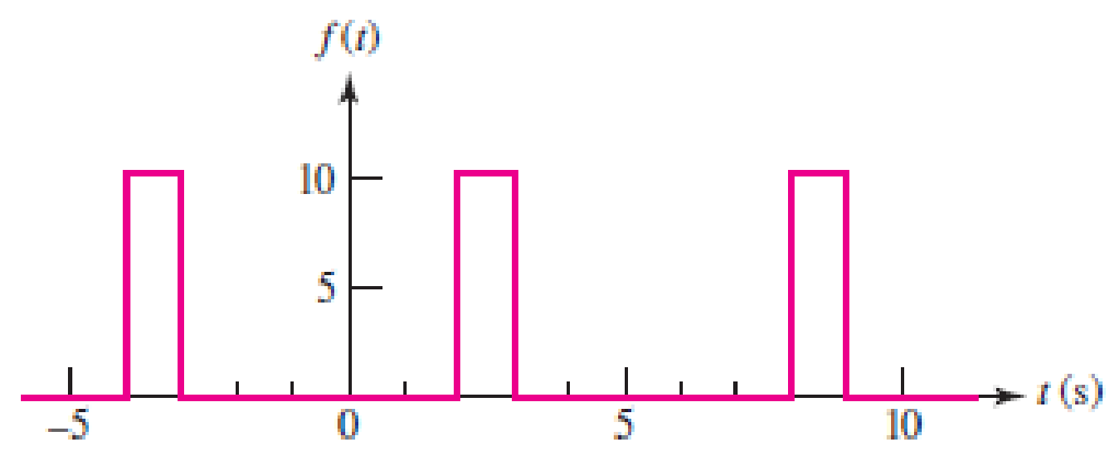
■ FIGURE 17.30
(a)
Sketch
Answer to Problem 8E
The sketch for
Explanation of Solution
Given data:
Refer to Figure 17.30 in the textbook.
Formula used:
Write the general expression for Fourier series expansion.
Write the general expression for Fourier series coefficient
Write the general expression for Fourier series coefficient
Write the general expression for Fourier series coefficient
Write the expression to calculate the fundamental angular frequency.
Here,
Calculation:
In the given Figure 17.29, the time period is
Substitute 6 for T in equation (5) to find
Substitute 6 for T in equation (2) to find the value of coefficient
Simplify the above equation as follows,
Substitute 6 for T in equation (3) to find the value of coefficient
The above equation as follows,
Substitute equation (6) in equation (7) as follows,
Now finding the Fourier coefficient
Substitute 6 for T in equation (4) to find the value of coefficient
The above equation as follows,
Substitute equation (6) in equation (9) as follows,
Substituting the value of
The function
For
Therefore, equation (11) will be as follows,
Simplify the above equation as follows,
Similarly, for
Therefore, equation (11) will be as follows,
From equation (12), the above equation is written as,
Similarly, for
Therefore, equation (11) will be as follows,
From equation (13), the above equation is written as,
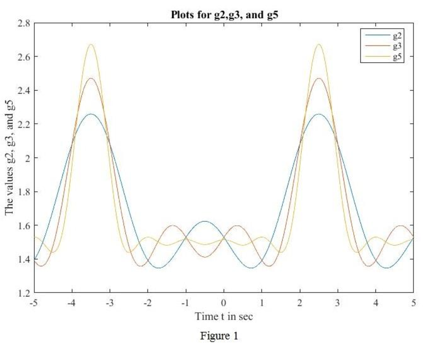
MATLAB code to sketch for
t=-5:0.01:5;
g2=1.667-0.275*cos(3.141*t/3)+0.159*sin(3.141*t/3)+0.137*cos(2*3.141*t/3)-0.238*sin(2*3.141*t/3);
g3=1.667-0.275*cos(3.141*t/3)+0.159*sin(3.141*t/3)+0.137*cos(2*3.141*t/3)-0.238*sin(2*3.141*t/3)+0.212*sin(pi*t);
g5=1.667- 0.275*cos(3.141*t/3)+0.159*sin(3.141*t/3)+0.137*cos(2*3.141*t/3)-0.238*sin(2*3.141*t/3)+0.212*sin(pi*t)-0.069*cos(4*pi*t/3)-0.119*sin(4*pi*t/3)+0.055*cos(5*pi*t/3)+0.0318*sin(5*pi*t/3);
plot(t,g2,t,g3,t,g5)
legend({'g2','g3','g5'},'Location','best')
xlabel('Time t in sec')
ylabel('The values g2, g3, and g5')
title('Plots for g2,g3, and g5')
MATLAB output: The MATLAB output shown in Figure 1.
MATLAB code to sketch for
t=linspace(-5,5,1000); % vector for time over 1000 points.
T=6; % Period
w0=2*pi/T; % natural frequency, is w0=2*pi.
f0=1.667; % constant.
N=40;
for i=1:1000;
sum=0;
for n=1:N;
sum=sum+(1/n*pi)*(sin(n*pi) -sin(2*n*pi/3))*cos(n*pi*t(i)/3) + (1/n*pi)*(cos(2*n*pi/3) -cos(n*pi))*sin(n*pi*t(i)/3);
end
f40(i)=f0+sum;
end
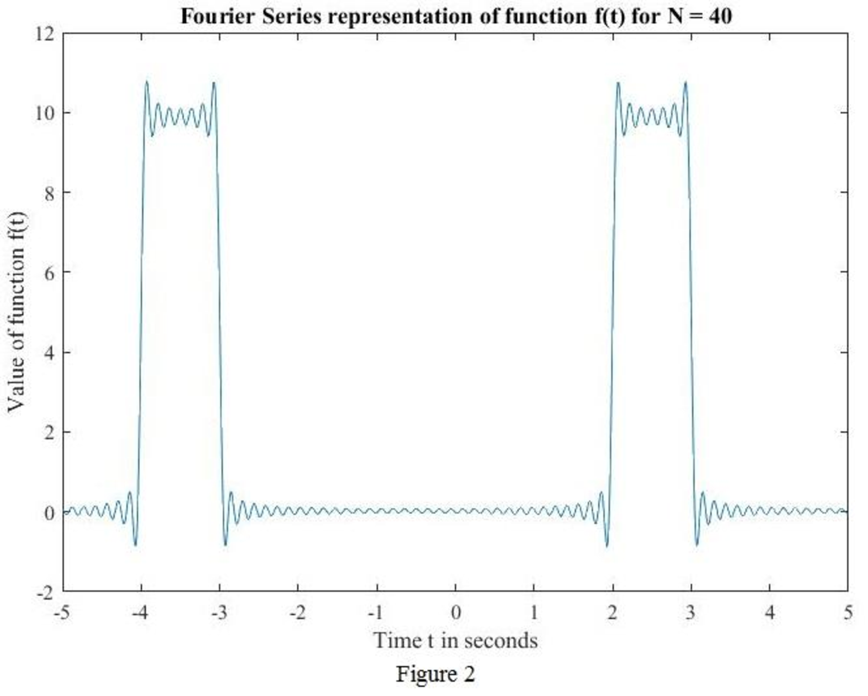
plot(t,f40)
xlabel('Time t in seconds')
ylabel('Value of function f(t)')
plot_ttle = ['Fourier Series representation of function f(t) for N = ',num2str(N)];
title(plot_ttle);
MATLAB output: The MATLAB output shown in Figure 2.
MATLAB code to sketch for
t=linspace(-5,5,1000); % vector for time over 1000 points.
T=6; % Period
w0=2*pi/T; % natural frequency, is w0=2*pi.
f0=1.667; % constant.
N=40; % consider N=40 for instant.
for i=1:1000;
g2=1.667-0.275*cos(3.141*t(i)/3)+0.159*sin(3.141*t(i)/3)+0.137*cos(2*3.141*t(i)/3)-0.238*sin(2*3.141*t(i)/3);
g3=1.667-0.275*cos(3.141*t(i)/3)+0.159*sin(3.141*t(i)/3)+0.137*cos(2*3.141*t(i)/3)-0.238*sin(2*3.141*t(i)/3)+0.212*sin(pi*t(i));
g5=1.667-0.275*cos(3.141*t(i)/3)+0.159*sin(3.141*t(i)/3)+0.137*cos(2*3.141*t(i)/3)-0.238*sin(2*3.141*t/3)+0.212*sin(pi*t)-0.069*cos(4*pi*t(i)/3)-0.119*sin(4*pi*t(i)/3)+0.055*cos(5*pi*t(i)/3)+0.0318*sin(5*pi*t(i)/3);
end
for i=1:1000;
sum=0;
for n=1:N;
sum=sum+(1/n*pi)*(sin(n*pi) -sin(2*n*pi/3))*cos(n*pi*t(i)/3) + (1/n*pi)*(cos(2*n*pi/3) -cos(n*pi))*sin(n*pi*t(i)/3);
end
f40(i)=f0+sum;
end
plot(t,g2,t,g3,t,g5,t,f40)
legend({'g2','g3','g5','f40'},'Location','best')
xlabel('Time t in sec')
ylabel('The values g2, g3, g5 and f40')
title('Plots for g2, g3, g5 and f40')
MATLAB output:
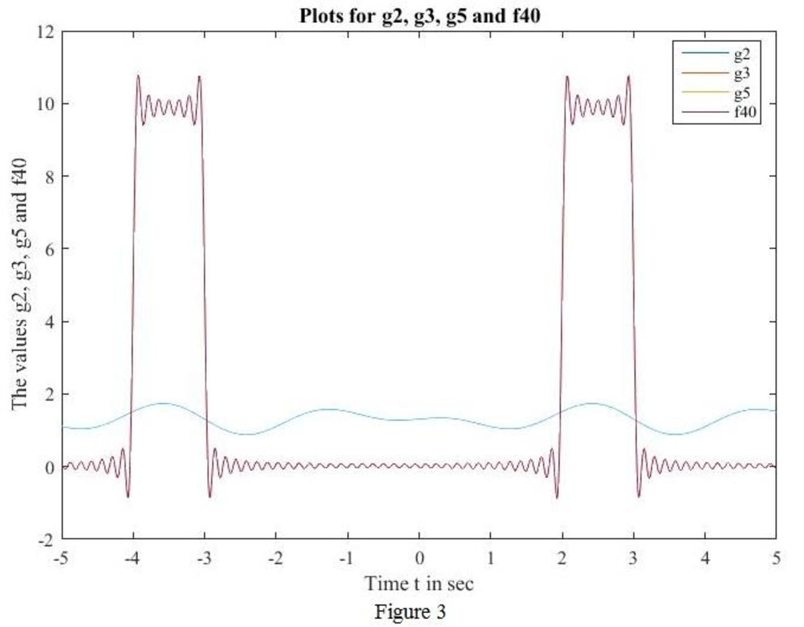
Conclusion:
Thus, the sketch for
(b)
Find the function
Answer to Problem 8E
The value of
Explanation of Solution
Given data:
Refer to Figure 17.30 in the textbook.
Calculation:
From Part (a), the function
Finding
From Part (a),
Finding
From Part (a),
Finding
From Part (a),
Finding
Conclusion:
Thus, the value of
Want to see more full solutions like this?
Chapter 17 Solutions
Loose Leaf for Engineering Circuit Analysis Format: Loose-leaf
Additional Engineering Textbook Solutions
Electrical Engineering: Principles & Applications (7th Edition)
Programmable Logic Controllers
Microelectronics: Circuit Analysis and Design
Basic Engineering Circuit Analysis
ELECTRICITY FOR TRADES (LOOSELEAF)
ANALYSIS+DESIGN OF LINEAR CIRCUITS(LL)


- Let's examine the function g(t)= {Go for - π < t < -( π/2), {-Go for -( π/2) < t < ( π/2), {Go for ( π/2) < t < π, which is characterized by being 2 π-periodic. Firstly, without mathematical calculations, clarify why every bn value must be 0. Secondly, sketch the g(t) graph within the range of [-4 π,4 π]. Thirdly, express the Fourier expansion of g(t). Lastly, plot the g(t) using the first 3, 5, 10, 15, 20, and 25 terms of the series. At what point does the graph start resembling your initial sketch in the first question?arrow_forwardFind the Fourier series representation of f(t) = 1 + t, −π < t < π , period 2π .arrow_forwardQ1/Obtain the Fourier Transform to the rectangular pulse of duration 2 second and having a magnitude of 10 volts. 2/Find the Fourier series for the periodic function giving below: x (t) (cosx, 0, {cos 0 <x <1 T <x <2Tarrow_forward
- x [n] = [1,5,2,3,3,1,2,3]Find the Fourier coefficients for the discrete time signal given by the fast Fourier transform.arrow_forwardObtain the Fourier series expansion of the periodic function f(t) of period 2π defined by the given. Show your solution.arrow_forwardGiven the finite-duration sequence below, x[n]={-4,1,2,0,3} where -4 is when n=0, if it has a fourier transform of X(w) , what is the value of X(0)?arrow_forward
- Suppose there is a sequence x[n] = [2, -1, 0, c, 1] where the value of c is unknown. X[k] is the DFT of x[n]. Let Y[k] = X[k]exp(i6πk/5). The inverse fourier transform of Y is y[n] = [2, 1, 2, -1, 0]. What is the value of c?arrow_forwardobtain the Fourier transform of the signal as a single expressionarrow_forwardThe signal X(t)=(e^-bt) u(t) is given as input to a system with a unit impulse response h(t)=(e^-at) u(t). if a=2,b=1, Find the y(t) signal obtained at the output by the following methods.a. find by calculating the convolution of x(t) and h(t) in the form y(t) = x(t) ∗ h(t).b. find y(t) = F^-1{H(jw) X(jw)} by calculating the inverse Fourier Transform of the product of the Fourier transforms of x(t) and h(t). I used the ^ symbol for an exponential expressionarrow_forward
- Calculate the frequency bin width of a 1024-point Fourier vector for whichthe data is sampled at 512,000 Hz. Explain how the roots of unity are derived and how they are usedarrow_forwardQ/Obtain the Fourier Transform to the rectangular pulse of duration 2 second and having a magnitude of 10 volts. Q/Find the Fourier series for the periodic function giving below: x (t) (cosx, 0, {cos 0arrow_forwardQ/Obtain the Fourier Transform to the rectangular pulse of duration 2 second and having a magnitude of 10 volts.arrow_forward
 Introductory Circuit Analysis (13th Edition)Electrical EngineeringISBN:9780133923605Author:Robert L. BoylestadPublisher:PEARSON
 Delmar's Standard Textbook Of ElectricityElectrical EngineeringISBN:9781337900348Author:Stephen L. HermanPublisher:Cengage Learning
 Programmable Logic ControllersElectrical EngineeringISBN:9780073373843Author:Frank D. PetruzellaPublisher:McGraw-Hill Education
 Fundamentals of Electric CircuitsElectrical EngineeringISBN:9780078028229Author:Charles K Alexander, Matthew SadikuPublisher:McGraw-Hill Education
 Electric Circuits. (11th Edition)Electrical EngineeringISBN:9780134746968Author:James W. Nilsson, Susan RiedelPublisher:PEARSON
 Engineering ElectromagneticsElectrical EngineeringISBN:9780078028151Author:Hayt, William H. (william Hart), Jr, BUCK, John A.Publisher:Mcgraw-hill Education,