
Videos
Human blood behaves as a Newtonian fluid (see Prob. 20.55) in the high shear rate region where
where
|
|
0.91 | 3.3 | 4.1 | 6.3 | 9.6 | 23 | 36 | 49 | 65 | 105 | 126 | 215 | 315 | 402 |
|
|
0.059 | 0.15 | 0.19 | 0.27 | 0.39 | 0.87 | 1.33 | 1.65 | 2.11 | 3.44 | 4.12 | 7.02 | 10.21 | 13.01 |
| Region | Casson | Transition | Newtonian |
Find the values of
To calculate: The values of
| 0.91 | 3.3 | 4.1 | 6.3 | 9.6 | 23 | 36 | 49 | 65 | 105 | 126 | 215 | 315 | 402 | |
| 0.0059 | 0.15 | 0.19 | 0.27 | 0.39 | 0.84 | 1.33 | 1.65 | 2.11 | 3.44 | 4.12 | 7.02 | 10.21 | 13.01 | |
| Region | Casson | Transition | Newtonian | |||||||||||
Also, find the correlation coefficient for each regression analysis. Plot the two regression lines on the Casson plot (
) and extend the regressions lines as dashed lines into adjoining regressions and include the given data points in the plots.
Answer to Problem 15P
Solution: In the Casson region
and in Newtonian region
and in Newtonian region
Explanation of Solution
Given Information: Consider the experimentally measured values of
| 0.91 | 3.3 | 4.1 | 6.3 | 9.6 | 23 | 36 | 49 | 65 | 105 | 126 | 215 | 315 | 402 | |
| 0.0059 | 0.15 | 0.19 | 0.27 | 0.39 | 0.84 | 1.33 | 1.65 | 2.11 | 3.44 | 4.12 | 7.02 | 10.21 | 13.01 | |
| Region | Casson | Transition | Newtonian | |||||||||||
The Casson relationship is with
The relationship for the Newtonian fluid,
Formula used:
If
data points
Here,
If
data points
The correlation coefficient is,
Here,
Calculation:
Consider the experimentally measured values of
| 0.91 | 3.3 | 4.1 | 6.3 | 9.6 | 23 | 36 | 49 | 65 | 105 | 126 | 215 | 315 | 402 | |
| 0.0059 | 0.15 | 0.19 | 0.27 | 0.39 | 0.84 | 1.33 | 1.65 | 2.11 | 3.44 | 4.12 | 7.02 | 10.21 | 13.01 | |
| Region | Casson | Transition | Newtonian | |||||||||||
The Casson relationship is with
Defining the two variables
Therefore, the unknown constant
Construct the following table considering the data in the Casson regions to compute the unknown constant
| 1 | 0.91 | 0.0059 | 0.95394 | 0.07681 | 0.91000 | 0.07327 |
| 2 | 3.3 | 0.15 | 1.81659 | 0.38730 | 3.30000 | 0.70356 |
| 3 | 4.1 | 0.19 | 2.02485 | 0.43589 | 4.10000 | 0.88261 |
| 4 | 6.3 | 0.27 | 2.50998 | 0.51962 | 6.30000 | 1.30422 |
| 5 | 9.6 | 0.39 | 3.09839 | 0.62450 | 9.60000 | 1.93494 |
| 6 | 23 | 0.84 | 4.79583 | 0.91652 | 23.00000 | 4.39545 |
| 7 | 36 | 1.33 | 6.00000 | 1.15326 | 36.00000 | 6.91954 |
| 21.19957 | 4.11389 | 83.21000 | 16.21360 |
Therefore, the unknown constant
Therefore,
Hence, the linear regression line for Casson region is,
Construct the table to calculate the correlation coefficients defining
| 1 | 0.95394 | 0.07681 | 0.26101 | 0.17789 | 0.01022 |
| 2 | 1.81659 | 0.38730 | 0.04016 | 0.34830 | 0.00152 |
| 3 | 2.02485 | 0.43589 | 0.02305 | 0.38944 | 0.00216 |
| 4 | 2.50998 | 0.51962 | 0.00463 | 0.48527 | 0.00118 |
| 5 | 3.09839 | 0.62450 | 0.00135 | 0.60151 | 0.00053 |
| 6 | 4.79583 | 0.91652 | 0.10812 | 0.93682 | 0.00041 |
| 7 | 6.00000 | 1.15326 | 0.31986 | 1.17469 | 0.00046 |
| 0.75818 | 0.01648 |
Therefore,
Hence, the correlation coefficients,
Therefore, for Casson region the linear fit is,
And the correlation coefficients,
Consider the Newtonian relationship as,
From the linear regression,
Construct the following table considering the data in the Newton regions to compute the unknown constant
| 1 | 105 | 3.44 | 11025 | 361.20 |
| 2 | 126 | 4.12 | 15876 | 519.12 |
| 3 | 215 | 7.02 | 46225 | 1509.30 |
| 4 | 315 | 10.21 | 99225 | 3216.15 |
| 5 | 402 | 13.01 | 161604 | 5230.02 |
| 37.8 | 333955 | 10835.79 |
Therefore, the unknown constant
Therefore,
Hence, the linear regression line for Newtonian region is,
Construct the table to calculate the correlation coefficients defining
| 1 | 105 | 3.44 | 16.97440 | 3.40725 | 0.00107 |
| 2 | 126 | 4.12 | 16.97440 | 4.08870 | 0.00098 |
| 3 | 215 | 7.02 | 49.28040 | 6.97675 | 0.00187 |
| 4 | 315 | 10.21 | 104.24410 | 10.22175 | 0.00014 |
| 5 | 402 | 13.01 | 169.26010 | 13.04490 | 0.00122 |
| 356.73340 | 0.00528 |
Therefore,
Hence, the correlation coefficients,
Therefore, for Newtonian region the linear fit is
And the correlation coefficients,
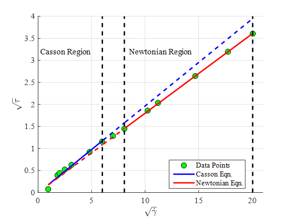
Graph:
Consider the two regression lines in the field of
In the Casson region,
In the Newtonian region,
Construct the MATLAB function ‘Code_97924_20_15a.m’ to plot the two regression lines on the Casson plot (
) and extend the regressions lines as dashed lines into adjoining regressions and include the given data points in the plots.
The comparison is shown on the plot as,
Want to see more full solutions like this?
Chapter 20 Solutions
Numerical Methods for Engineers


 Advanced Engineering MathematicsAdvanced MathISBN:9780470458365Author:Erwin KreyszigPublisher:Wiley, John & Sons, Incorporated
 Numerical Methods for EngineersAdvanced MathISBN:9780073397924Author:Steven C. Chapra Dr., Raymond P. CanalePublisher:McGraw-Hill Education
 Introductory Mathematics for Engineering Applicat...Advanced MathISBN:9781118141809Author:Nathan KlingbeilPublisher:WILEY
 Mathematics For Machine TechnologyAdvanced MathISBN:9781337798310Author:Peterson, John.Publisher:Cengage Learning,
