
Videos
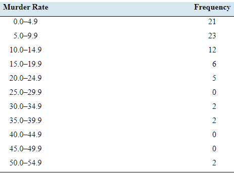
Murder, she wrote: The following frequency distribution presents the number of murders (including negligent manslaughter) per 100,000 population for each U.S. city with population over 250,000 in a recent year.
- How many classes are there?
- What is the class width?
- What are the class limits?
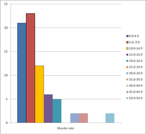
- Construct a frequency histogram.
- Construct a relative frequency distribution.
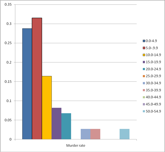
- Construct a relative frequency histogram.
- What percentage of cities had murder rates less than 10 per 100,000 population?
- What percentage of cities had murder rates of 30 or more per 100,000 population?
a.
To find:The number of classes.
Answer to Problem 28E
The number of classes is 11.
Explanation of Solution
Given information:The following frequency distribution presents the number of murders per 100,000 population of each U.S. city with population over 250,000 in a recent year.
| Murder rate | Frequency |
| 0.0-4.9 | 21 |
| 5.0-9.9 | 23 |
| 10-14.9 | 12 |
| 15.0-19.9 | 6 |
| 20.0-24.9 | 5 |
| 25.0-29.9 | 0 |
| 30.0-34.9 | 2 |
| 35.0-39.9 | 2 |
| 40.0-44.9 | 0 |
| 45.0-49.9 | 0 |
| 50.0-54.9 | 2 |
Definition used:The classes are intervals of equal width that cover all the values that are observed.
Calculation:
From the given table, the classes are
The number of classes is 11.
Hence, the number of classes is 11.
b.
To find:The class width.
Answer to Problem 28E
The class width is 5.
Explanation of Solution
Given information:The following frequency distribution presents the number of murders per 100,000 population of each U.S. city with population over 250,000 in a recent year.
| Murder rate | Frequency |
| 0.0-4.9 | 21 |
| 5.0-9.9 | 23 |
| 10-14.9 | 12 |
| 15.0-19.9 | 6 |
| 20.0-24.9 | 5 |
| 25.0-29.9 | 0 |
| 30.0-34.9 | 2 |
| 35.0-39.9 | 2 |
| 40.0-44.9 | 0 |
| 45.0-49.9 | 0 |
| 50.0-54.9 | 2 |
Formula used:
Calculation:
From the given table, the number of classes is 11.
The largest data value is 54.9 and the smallest data value is 0.0.
Thus, each class is an interval with equal width of 5.0.
Hence, the class width is 5.
c.
To find:The class limits.
Answer to Problem 28E
Lower limits: 0.0, 5.0, 10.0, 15.0, 20.0, 25.0, 30.0, 35.0, 40.0, 45.0, 50.0.
Upper limits: 4.9, 9.9, 14.9, 19.9, 24.9, 29.9, 34.9, 39.9, 44.9, 49.9, 54.9.
Explanation of Solution
Given information:The following frequency distribution presents the number of murders per 100,000 population of each U.S. city with population over 250,000 in a recent year.
| Murder rate | Frequency |
| 0.0-4.9 | 21 |
| 5.0-9.9 | 23 |
| 10-14.9 | 12 |
| 15.0-19.9 | 6 |
| 20.0-24.9 | 5 |
| 25.0-29.9 | 0 |
| 30.0-34.9 | 2 |
| 35.0-39.9 | 2 |
| 40.0-44.9 | 0 |
| 45.0-49.9 | 0 |
| 50.0-54.9 | 2 |
Definition used:
The lower class limit of a class is the smallest value
that can appear in that class.
The upper class limit of a class is the largest value that can appear in that class.
Calculation:
From the table, we can have the lower limits and upper limits are as follows:
Lower limits: 0.0, 5.0, 10.0, 15.0, 20.0, 25.0, 30.0, 35.0, 40.0, 45.0, 50.0.
Upper limits: 4.9, 9.9, 14.9, 19.9, 24.9, 29.9, 34.9, 39.9, 44.9, 49.9, 54.9.
d.
To construct: A frequency histogram.
Explanation of Solution
Given information:The following frequency distribution presents the number of murders per 100,000 population of each U.S. city with population over 250,000 in a recent year.
| Murder rate | Frequency |
| 0.0-4.9 | 21 |
| 5.0-9.9 | 23 |
| 10-14.9 | 12 |
| 15.0-19.9 | 6 |
| 20.0-24.9 | 5 |
| 25.0-29.9 | 0 |
| 30.0-34.9 | 2 |
| 35.0-39.9 | 2 |
| 40.0-44.9 | 0 |
| 45.0-49.9 | 0 |
| 50.0-54.9 | 2 |
Definition used: Histograms based on frequency distributions are called frequency histogram.
Solution:
The frequency histogram for the given data is given by
e.
To construct: A relative frequency distribution.
Explanation of Solution
Given information:The following frequency distribution presents the number of murders per 100,000 population of each U.S. city with population over 250,000 in a recent year.
| Murder rate | Frequency |
| 0.0-4.9 | 21 |
| 5.0-9.9 | 23 |
| 10-14.9 | 12 |
| 15.0-19.9 | 6 |
| 20.0-24.9 | 5 |
| 25.0-29.9 | 0 |
| 30.0-34.9 | 2 |
| 35.0-39.9 | 2 |
| 40.0-44.9 | 0 |
| 45.0-49.9 | 0 |
| 50.0-54.9 | 2 |
Formula used:
Solution:
From the given table,
The sum of all frequency is
The table of relative frequency is given by
| Murder rate | Frequency | Relative frequency |
| 0.0-4.9 | 21 | |
| 5.0-9.9 | 23 | |
| 10-14.9 | 12 | |
| 15.0-19.9 | 6 | |
| 20.0-24.9 | 5 | |
| 25.0-29.9 | 0 | |
| 30.0-34.9 | 2 | |
| 35.0-39.9 | 2 | |
| 40.0-44.9 | 0 | |
| 45.0-49.9 | 0 | |
| 50.0-54.9 | 2 |
f.
To construct: A relative frequency histogram.
Explanation of Solution
Given information:The following frequency distribution presents the number of murders per 100,000 population of each U.S. city with population over 250,000 in a recent year.
| Murder rate | Frequency |
| 0.0-4.9 | 21 |
| 5.0-9.9 | 23 |
| 10-14.9 | 12 |
| 15.0-19.9 | 6 |
| 20.0-24.9 | 5 |
| 25.0-29.9 | 0 |
| 30.0-34.9 | 2 |
| 35.0-39.9 | 2 |
| 40.0-44.9 | 0 |
| 45.0-49.9 | 0 |
| 50.0-54.9 | 2 |
Definition used: Histograms based on relative frequency distributions are called relative frequency histogram.
Solution:
| Murder rate | Relative frequency |
| 0.0-4.9 | 0.288 |
| 5.0-9.9 | 0.315 |
| 10-14.9 | 0.164 |
| 15.0-19.9 | 0.082 |
| 20.0-24.9 | 0.068 |
| 25.0-29.9 | 0 |
| 30.0-34.9 | 0.027 |
| 35.0-39.9 | 0.027 |
| 40.0-44.9 | 0 |
| 45.0-49.9 | 0 |
| 50.0-54.9 | 0.027 |
Therelative frequency histogram for the given data is given by
g.
To find: The percentage of cities had murder rates less than 10 per 100,00
0 population.
Answer to Problem 28E
The percentage of cities had murder rates less than 10 per 100,000 population.is 60.3%.
Explanation of Solution
Given information:The following frequency distribution presents the number of murders per 100,000 population of each U.S. city with population over 250,000 in a recent year.
| Murder rate | Frequency |
| 0.0-4.9 | 21 |
| 5.0-9.9 | 23 |
| 10-14.9 | 12 |
| 15.0-19.9 | 6 |
| 20.0-24.9 | 5 |
| 25.0-29.9 | 0 |
| 30.0-34.9 | 2 |
| 35.0-39.9 | 2 |
| 40.0-44.9 | 0 |
| 45.0-49.9 | 0 |
| 50.0-54.9 | 2 |
Calculation:
The relative frequency table is given by
| Murder rate | Relative frequency |
| 0.0-4.9 | 0.288 |
| 5.0-9.9 | 0.315 |
| 10-14.9 | 0.164 |
| 15.0-19.9 | 0.082 |
| 20.0-24.9 | 0.068 |
| 25.0-29.9 | 0 |
| 30.0-34.9 | 0.027 |
| 35.0-39.9 | 0.027 |
| 40.0-44.9 | 0 |
| 45.0-49.9 | 0 |
| 50.0-54.9 | 0.027 |
From the above data, the relative frequencies of murder rates less than 10 per 100,000 populationare 0.288 and 0.315
The sum of all the above relative frequencies is
Then, its percentage is 60.3%
Hence, the percentage of cities had murder rates less than 10 per 100,000 population.is 60.3%.
h.
To find: The percentage of cities had murder rates of 30 or more per 100,000 populations.
Answer to Problem 28E
The percentage of cities had murder rates of 30 or more per 100,000 populations is 8.1%.
Explanation of Solution
Given information:The following frequency distribution presents the number of murders per 100,000 population of each U.S. city with population over 250,000 in a recent year.
| Murder rate | Frequency |
| 0.0-4.9 | 21 |
| 5.0-9.9 | 23 |
| 10-14.9 | 12 |
| 15.0-19.9 | 6 |
| 20.0-24.9 | 5 |
| 25.0-29.9 | 0 |
| 30.0-34.9 | 2 |
| 35.0-39.9 | 2 |
| 40.0-44.9 | 0 |
| 45.0-49.9 | 0 |
| 50.0-54.9 | 2 |
Calculation:
The relative frequency table is given by
| Murder rate | Relative frequency |
| 0.0-4.9 | 0.288 |
| 5.0-9.9 | 0.315 |
| 10-14.9 | 0.164 |
| 15.0-19.9 | 0.082 |
| 20.0-24.9 | 0.068 |
| 25.0-29.9 | 0 |
| 30.0-34.9 | 0.027 |
| 35.0-39.9 | 0.027 |
| 40.0-44.9 | 0 |
| 45.0-49.9 | 0 |
| 50.0-54.9 | 0.027 |
From the above data, the relative frequencies of murder rates of 30 or more per 100,000 populationsare 0.027, 0.027, 0, 0 and 0.027.
The sum of all the above relative frequencies is
Then, its percentage is 8.1%
Hence, the percentage of cities had murder rates of 30 or more per 100,000 populations is 8.1%.
Want to see more full solutions like this?
Chapter 2 Solutions
Elementary Statistics 2nd Edition


 Glencoe Algebra 1, Student Edition, 9780079039897...AlgebraISBN:9780079039897Author:CarterPublisher:McGraw Hill