
a.The level of change in real
b. The level of change in real government spending and real taxes over the four most recent quarters of data available and the four quarters prior to that.
c. Provide the explanation to answer part a and part b using the IS and AD curves
Explanation of Solution
a. Real GDP: Real Gross Domestic Product
Real Government Expenditure: Real Government Spending
PCE: Personal Consumption Expenditure
[of a quarter of current year w.r.t to the prior quarter of previous year]
b.
[of a quarter of current year w.r.t to the prior quarter of previous year]
[of a quarter of current year w.r.t to the prior quarter of previous year]
| Year
Quarter Month | Real Govt. Spending | Change In Levels of Govt. Spend. | Level of Change in Real Govt Spend % | Real GDP | Change in Levels of GDP | Level of Change in Real GDP % | Federal Govt. Current Taxes Receipts | PCE | Real Taxes =Taxes/PCE * 100 | Level of Change in Real Taxes | Level of Change in Real Taxes % | ||
| 2016 Q1 Jan | 2903.1 | 16571.5 | 2060 | 109.9 | 1874.43 | ||||||||
| 2016 Q2 apr | 2896.3 | 16663.5 | 2096.2 | 110.5 | 1897.01 | ||||||||
| 2016 Q3 July | 2899.9 | 16778.1 | 2131.5 | 111 | 1920.27 | ||||||||
| 2016 Q4 oct | 2901.1 | 16851.4 | 2112.9 | 111.5 | 1894.98 | ||||||||
| 2017 Q1 jan | 2896.6 | -6.5 | -0.22 | 16903.2 | 331.7 | 2.00 | 2133.3 | 112.1 | 1903.03 | 28.60 | 1.53 | ||
| 2017 Q2 apr | 2895.2 | -1.1 | -0.04 | 17031 | 367.5 | 2.21 | 2150.6 | 112.2 | 1916.76 | 19.74 | 1.04 | ||
| 2017 Q3 july | 2899.9 | 0 | 0.00 | 17163.8 | 385.7 | 2.30 | 2176.7 | 112.6 | 1933.13 | 12.86 | 0.67 | ||
| 2017 Q4 oct | 2921.5 | 20.4 | 0.70 | 17286.4 | 435 | 2.58 | No data | 113.4 | No data | No data | No data |
*St. Louis Reserve Fred Database
Interpretation: Findings -
- Real Government Spending is increasing
- Real GDP is increasing
- Real Taxes are reducing
b. Graphs:
Fig1: Effect of Changes in Government Spending & Taxes On Shifts on Aggregate Demand Curve
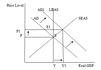
Short Run Upward moving
Fig2: Effect of Changes in Government Spending & Taxes On Shifts in IS Curve [Investment Saving Curve]
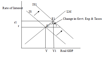
Short run equilibrium is attained between interest rates and output when IS intersects LM curves at point E. Here, Gross domestic product (GDP), or (Y), is placed on the horizontal axis, increasing as it stretches to the right. The nominal interest rate, or (i or R), makes up the vertical axis. If there is an increase in real government spending then the IS curve would shift to the right. ie. when the government spending goes up [when G goes up] it would shift the IS curve to the right and a new equilibrium is achieved at point E1. In the same way, reduction in taxes also causes the IS curve to shift rightward leading to new equilibrium rate of interest and real GDP. This causes an increase in the rate of interest and real GDP as found in the above table.
Introduction:
AD [Aggregate Demand] curve represents the relationship between the inflation rate &
The IS-LM model, which stands for "investment-savings, liquidity-money," is a Keynesian
Want to see more full solutions like this?
Chapter 23 Solutions
Economics of Money, Banking and Financial Markets, The, Business School Edition (5th Edition) (What's New in Economics)


 Principles of Economics (12th Edition)EconomicsISBN:9780134078779Author:Karl E. Case, Ray C. Fair, Sharon E. OsterPublisher:PEARSON
 Engineering Economy (17th Edition)EconomicsISBN:9780134870069Author:William G. Sullivan, Elin M. Wicks, C. Patrick KoellingPublisher:PEARSON
 Principles of Economics (MindTap Course List)EconomicsISBN:9781305585126Author:N. Gregory MankiwPublisher:Cengage Learning
 Managerial Economics: A Problem Solving ApproachEconomicsISBN:9781337106665Author:Luke M. Froeb, Brian T. McCann, Michael R. Ward, Mike ShorPublisher:Cengage Learning
 Managerial Economics & Business Strategy (Mcgraw-...EconomicsISBN:9781259290619Author:Michael Baye, Jeff PrincePublisher:McGraw-Hill Education