
ELEM. STATISTICS TEXT W/ MANUAL+CONNECT
1st Edition
ISBN: 9781260722031
Author: Navidi
Publisher: McGraw-Hill Publishing Co.
expand_more
expand_more
format_list_bulleted
Concept explainers
Videos
Textbook Question
Chapter 2.4, Problem 13E
College degrees: Both of the following time-series plots present the percentage of U.S. adults who have earned college degrees during the years 2007—20 15.
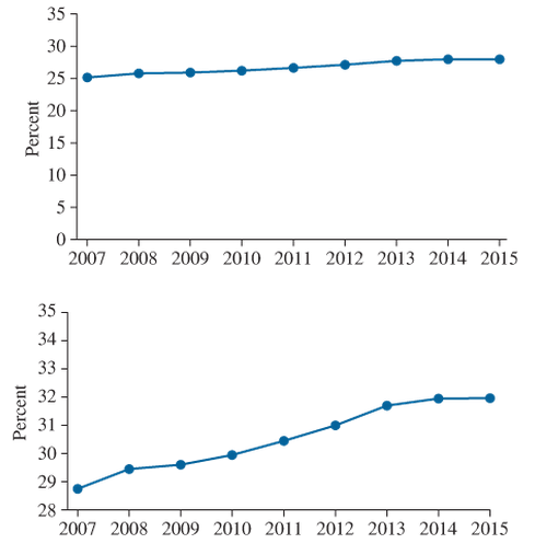
Which of the following statements is true and why?
- The percentage of U.S. adults with college degrees increased slightly between 2007 and 2015.
- The percentage of U.S. adults with college degrees increased considerably between 2007 and 2015.
Expert Solution & Answer
Want to see the full answer?
Check out a sample textbook solution
Students have asked these similar questions
In general, ___________% of the values in a data set lie at or below the 28
th
percentile.
_______________ % of the values in a data set lie at or above the 90
th
percentile..
If a sample consists of 700 test scores, _________of them would be
at or below
the 52
th
percentile.
If a sample consists of 700 test scores, ________ of them would be
at or above
the 64
th
percentile.
A company with a high operating leverage will experience which of the following?
a) the same percentage change in operating income as a result of a percentage change in sales.
b) a small percentage change in operating income as a result of a small percentage change in sales.
c) a large percentage change in operating income as a result of a small percentage change in sales.
d) a small percentage change in operating income as a result of a large percentage change in sales.
The median home value in West Virginia and Kentucky (adjusted for inflation) are shown below.
Year
West Virginia
Kentucky
1950
33200
32000
2000
72800
86700
If we assume that the house values are changing linearly,a) In which state have home values increased at a higher rate? b) If these trends were to continue, what would be the median home value in West Virginia in 2010?$ c) If we assume the linear trend existed before 1950 and continues after 2000, the two states' median house values will be (or were) equal in what year? (The answer might be absurd)The year
Chapter 2 Solutions
ELEM. STATISTICS TEXT W/ MANUAL+CONNECT
Ch. 2.1 - In Exercises 5-8, fill in each blank with the...Ch. 2.1 - In Exercises 5-8, fill in each blank with the...Ch. 2.1 - In Exercises 5-8, fill in each blank with the...Ch. 2.1 - In Exercises 5-8, fill in each blank with the...Ch. 2.1 - In Exercises 9—12, determine whether the...Ch. 2.1 - In Exercises 9—12, determine whether the...Ch. 2.1 - In Exercises 9—12, determine whether the...Ch. 2.1 - In Exercises 9—12, determine whether the...Ch. 2.1 - The following bar graph presents the average...Ch. 2.1 - The most common blood typing system divides human...
Ch. 2.1 - Following is a pie chart that presents the...Ch. 2.1 - Government spending: The following pie chart...Ch. 2.1 - U.S. population: The following side-by-side bar...Ch. 2.1 - Super Bowl: The following side-by-side bar graph...Ch. 2.1 - Smartphone sales: The following frequency...Ch. 2.1 - Popular video games: The following frequency...Ch. 2.1 - More smartphones: Using the data in Exercise 19:...Ch. 2.1 - More video games: Using the data in Exercise 20:...Ch. 2.1 - Hospital admissions: The following frequency...Ch. 2.1 - World population: Following are the populations of...Ch. 2.1 - Ages of video garners: The Nielsen Company...Ch. 2.1 - How secure is your job? In a survey, employed...Ch. 2.1 - Back up your data: In a survey commissioned by the...Ch. 2.1 - Education levels: The following frequency...Ch. 2.1 - Twitter followers: The following frequency...Ch. 2.1 - Music sales: The following frequency distribution...Ch. 2.1 - Keeping up with the Kardashians: The following...Ch. 2.1 - Bought a new car lately? The following table...Ch. 2.1 - Bought a new- truck lately? The following table...Ch. 2.1 - Happy Halloween: The following table presents...Ch. 2.1 - Native languages: The following frequency...Ch. 2.1 - Proportion of females: Following are the...Ch. 2.2 - Prob. 5ECh. 2.2 - In Exercises 5—8, fill in each blank with the...Ch. 2.2 - In Exercises 5—8, fill in each blank with the...Ch. 2.2 - In Exercises 5—8, fill in each blank with the...Ch. 2.2 - In Exercises 9—12, determine whether the...Ch. 2.2 - In Exercises 9—12, determine whether the...Ch. 2.2 - In Exercises 9—12, determine whether the...Ch. 2.2 - In Exercises 9—12, determine whether the...Ch. 2.2 - In Exercises 13—16, classify the histogram as...Ch. 2.2 - In Exercises 13—16, classify the histogram as...Ch. 2.2 - In Exercises 13—16, classify the histogram as...Ch. 2.2 - In Exercises 13—16, classify the histogram as...Ch. 2.2 - In Exercises 17 and 18, classify the histogram as...Ch. 2.2 - In Exercises 17 and 18, classify the histogram as...Ch. 2.2 - Student heights: The following frequency histogram...Ch. 2.2 - Trained rats: Forty rats were trained to run a...Ch. 2.2 - Cholesterol: The following histogram shows the...Ch. 2.2 - Blood pressure: The following histogram shows the...Ch. 2.2 - Olympic athletes: The following frequency...Ch. 2.2 - Hows the weather? The following relative frequency...Ch. 2.2 - Skewed which way? For which of the following data...Ch. 2.2 - Skewed which way? For which of the following data...Ch. 2.2 - Batting average: The following frequency...Ch. 2.2 - Batting average: The following frequency...Ch. 2.2 - Time spent playing video games: A sample of 200...Ch. 2.2 - Murder, she wrote: The following frequency...Ch. 2.2 - BMW prices: The following table presents the...Ch. 2.2 - Geysers: The geyser Old Faithful in Yellowstone...Ch. 2.2 - Hail to the chief: There have been 58 presidential...Ch. 2.2 - Internet radio: The following table presents the...Ch. 2.2 - Brothers and sisters: Thirty students in a...Ch. 2.2 - Cough, cough: The following table presents the...Ch. 2.2 - Prob. 37ECh. 2.2 - Prob. 38ECh. 2.2 - Prob. 39ECh. 2.2 - Prob. 40ECh. 2.2 - Frequency polygon: Using the data in Exercise 29:...Ch. 2.2 - Prob. 42ECh. 2.2 - Ogive: Using the data in Exercise 27: Compute the...Ch. 2.2 - Ogive: Using the data in Exercise 28: Compute the...Ch. 2.2 - Ogive: Using the data in Exercise 29: Compute the...Ch. 2.2 - Prob. 46ECh. 2.2 - Prob. 47ECh. 2.2 - Prob. 48ECh. 2.2 - Prob. 49ECh. 2.2 - Prob. 50ECh. 2.2 - Prob. 51ECh. 2.2 - Prob. 52ECh. 2.2 - Frequencies and relative frequencies: The...Ch. 2.3 - In Exercises 3—6, fill in each blank with the...Ch. 2.3 - In Exercises 3—6, fill in each blank with the...Ch. 2.3 - In Exercises 3—6, fill in each blank with the...Ch. 2.3 - In Exercises 3—6, fill in each blank with the...Ch. 2.3 - Prob. 7ECh. 2.3 - In Exercises 7—10, determine whether the...Ch. 2.3 - In Exercises 7—10, determine whether the...Ch. 2.3 - In Exercises 7—10, determine whether the...Ch. 2.3 - Construct a stem-and-leaf plot for the following...Ch. 2.3 - Construct a stem-and-leaf plot for the following...Ch. 2.3 - List the data in the following stem-and-leaf plot....Ch. 2.3 - List the data in the following stein-and-leaf...Ch. 2.3 - Construct a dotplot for the data in Exercise 11.Ch. 2.3 - Prob. 16ECh. 2.3 - BMW prices: The following table presents the...Ch. 2.3 - Hows the weather? The following table presents the...Ch. 2.3 - Air pollution: The following table presents...Ch. 2.3 - Technology salaries: The following table presents...Ch. 2.3 - Tennis and golf: Following are the ages of the...Ch. 2.3 - Pass the popcorn: Following are the running times...Ch. 2.3 - More weather: Construct a dotplot for the data in...Ch. 2.3 - Prob. 24ECh. 2.3 - Looking for a job: The following table presents...Ch. 2.3 - Prob. 26ECh. 2.3 - Military spending: The following table presents...Ch. 2.3 - Prob. 28ECh. 2.3 - Dining out: The following time-series plot...Ch. 2.3 - Prob. 30ECh. 2.3 - Prob. 31ECh. 2.3 - More gold: The following time series plot presents...Ch. 2.3 - Prob. 33ECh. 2.3 - Prob. 34ECh. 2.3 - Vote: The following time-series plot presents the...Ch. 2.3 - Arctic ice sheet: The following table presents the...Ch. 2.3 - Prob. 37ECh. 2.4 - In Exercises 3 and 4, fill in each blank with the...Ch. 2.4 - In Exercises 3 and 4, fill in each blank with the...Ch. 2.4 - CD sales decline: Sales of CDs have been declining...Ch. 2.4 - Music sales: The following time-series plot and...Ch. 2.4 - Stock market prices: The Dow Jones Industrial...Ch. 2.4 - Save your money: In 2007, U.S. residents saved...Ch. 2.4 - Ill take mine with mustard: The following bar...Ch. 2.4 - Stream or download? The following bar graph...Ch. 2.4 - Female senators: Of the 100 members of the United...Ch. 2.4 - Age at marriage: Data compiled by the U.S. Census...Ch. 2.4 - College degrees: Both of the following time-series...Ch. 2.4 - Food expenditures: Both of the following...Ch. 2.4 - Prob. 15ECh. 2 - Following is the list of letter grades for...Ch. 2 - Prob. 2CQCh. 2 - Construct a frequency bar graph for the data in...Ch. 2 - Prob. 4CQCh. 2 - Prob. 5CQCh. 2 - Prob. 6CQCh. 2 - Prob. 7CQCh. 2 - Prob. 8CQCh. 2 - Prob. 9CQCh. 2 - Prob. 10CQCh. 2 - Following are the prices (in dollars) for a sample...Ch. 2 - Prob. 12CQCh. 2 - Prob. 13CQCh. 2 - Prob. 14CQCh. 2 - Prob. 15CQCh. 2 - Trust your doctor: The General Social Survey...Ch. 2 - Internet browsers: The following relative...Ch. 2 - Prob. 3RECh. 2 - Prob. 4RECh. 2 - Prob. 5RECh. 2 - House freshmen: Newly elected members of the U.S....Ch. 2 - More freshmen: For the data in Exercise 6:...Ch. 2 - Royalty: Following are the ages at death for all...Ch. 2 - Prob. 9RECh. 2 - Prob. 10RECh. 2 - Prob. 11RECh. 2 - Prob. 12RECh. 2 - Prob. 13RECh. 2 - Prob. 14RECh. 2 - Prob. 15RECh. 2 - Explain why the frequency bar graph and the...Ch. 2 - Prob. 2WAICh. 2 - Prob. 3WAICh. 2 - Prob. 4WAICh. 2 - Prob. 5WAICh. 2 - In the chapter introduction, we presented gas...Ch. 2 - In the chapter introduction, we presented gas...Ch. 2 - In the chapter introduction, we presented gas...Ch. 2 - Prob. 4CSCh. 2 - In the chapter introduction, we presented gas...Ch. 2 - Prob. 6CSCh. 2 - In the chapter introduction, we presented gas...Ch. 2 - Prob. 8CSCh. 2 - In the chapter introduction, we presented gas...
Knowledge Booster


Learn more about
Need a deep-dive on the concept behind this application? Look no further. Learn more about this topic, statistics and related others by exploring similar questions and additional content below.Similar questions
- If all positions were paid equally, how much would Switzerland spend on wages for data processing in a year? A) CHF 1.03 billion B) CHF 3.45 billion C) CHF 162.5 billion D) CHF 103.9 billion E) CHF 188.5 billion Transcribed Image Text:Likelihood of industries becoming automated in the future Proportion of jobs and their risk of automation. Note: the graph shows a linear decrease in the proportion of jobs at risk of full automation. 60% 55% 50% 45% 40% 35% 30% 25% 20% 15% 10% 5% 0% LLL H Retail Waste Management Transportation and Storage Technical feasibility of job automation Likelihood of automating job tasks Predictable Physical Work Data Processing Data Collection Unpredictable Physical Work Stakeholder Interactions Applying Expertise with Clients Managing Others 0% Finance and Insurance Proportion of Jobs at Risk of Full Automation Employment Share of Total Jobs 5% 10% 15% Manufacturing 20% 25% 30% % of Tasks which could be Automated 35% Administration 40% 45% 50% 55%…arrow_forwardAjax has established a new sandwich shop format for airports and train stations.Here, the sandwitches are only made from a specially made,long,individual loaf of bread.But the innovations is that the sandwiches are not made ahead in large batches.Intead,a few of each variety of sandwich are made at a time,in the shop,with the result being a better ability to exactly match supply to demand. If prior to this change the shop has roughly 5 percent leftovers of one-half of the sandwich varieties each day,but could have sold 10 percent more of the two best sellers that day,what are the potential benefits of the new format if the store sells 12 different sandwiches each with an average demand of 20 per day?arrow_forwardWhat is the ratio of the total jobs at risk in Transportation and Storage to those at riks in Retail? A) 4.68:7.79 B) 7.79:4.68 C) 52:41 D) 9:19 E) 30:27 Transcribed Image Text:Likelihood of industries becoming automated in the future Proportion of jobs and their risk of automation. Note: the graph shows a linear decrease in the proportion of jobs at risk of full automation. 60% 55% 50% 45% 40% 35% 30% 25% 20% 15% 10% 5% 0% Transportation and Storage Series Value Proportion of Jobs at Risk of Full Automation 52% Employment Share of Total Jobs Waste Management Transportation and 9% Manufacturing Retail Administration Finance and Insurance ch Other Electricity and Gas Transcribed Image Text:Likelihood of industries becoming automated in the future Proportion of jobs and their risk of automation. Note: the graph shows a linear decrease in the proportion of jobs at risk of full automation. 60% 55% 50% 45% 40% 35% 30% 25% 20% 15% 10% 5% 0% Waste Management Transportation and Retail…arrow_forward
- 12- Year 2000 2001 2002 2003 2004 2005 Sales 25 50 75 25 50 34 Calculate the third three years moving average from the above data. a. 75 b. 25 c. 50 d. Allarrow_forwardPrices of a particular commodity in five years in two cities are given below. Which city has more stable prices? Price in City A : 20 22 19 23 16Price in City B : 10 20 18 12 15arrow_forwardWhich of the following time periods will have the largest annual average increase in the percentage of jobs that could be fully automated (based on the provided images attached)? A) 2020-2028 B) 2028-2030 C) 2030-2035 D) 2035-2040 E) 2040-2050 Transcribed Image Text:Preparing for Automation The possibility of having robots or mechanical assistants completing our laborious, dangerous, or repetitive day-to-day tasks has long been a dream of humanity. Now, as Robotic Process Automation (RPA) becomes commonplace, this dream or concern, depending on viewpoint - is getting closer. RPA, far from the walking, talking android commonly found in science fiction series, can be thought of as a programmable piece of software which, through using a series of rules, will complete repetitive tasks with a lower error rate and less interruption than a human completing the same tasks. The aim of RPA, beyond improving efficiency, is to free up humans from the monotony of roles like data entry, stock…arrow_forward
- An electronic appliance manufacturer wants to know if there is a relationship between percentage change in deposable personal income which is reported quarterly by the government, and the percentage change in appliances sold by the manufacturer following same years of quarterly data. Brenda Chee and Clarence Paulus lead an analyst team has obtained data for the past 10 quarters. (Hint: Provides your answers in two decimal points) Quarter Percent change in income Percent Change in appliance sold Quarter Percent change in income Percent change in appliance sold 1 -2.3 -2.5 6 -1.0 1.0 2 -1.5 -1.0 7 0.7 1.4 3 2.8 7.4 8 5.2 3.4 4 0.5 2.6 9 -2.5 -0.5 5 4.6 8.5 10 1.7 1.8 (a) What forecasting model should be used for this data. Why?(5(b) Develop the forecasting model that you have proposed in (a).(c) Compute the relationship for these data. In your opinion, is the relationship between independentvariable…arrow_forwardQUESTION 3 Consider the basic food items consumed by a rural household: Food item Consumption Price (N$) June 2021 July 2021 June 2021 July 2021 Bread(loaves) 25 26 10.30 10.70 Cooking oil(litres) 5 6 45.00 59.40 Rice(kg) 10 8 34.50 36.20 Meat(kg) 15 16 88.90 92.20 Required to: a)Which food item has had the lowest relative quantity of consumption increase between the months of June and July? b) Which food item has had the lowest relative price increase between the months Juneand July 2021? c) Calculate and interpret a Paasche quantity index for July 2021.arrow_forwardIn a table of “Sales as a % of Moving Average” over a 5-year period the adjusted average of the four entries for Quarter I is 160 (the seasonal index for Quarter 1). Actual sales in Quarter 1 were 4000 dollars. What is the de-seasonalized value of sales in Quarter 1? _____arrow_forward
- The price (in rands) in June of a 1 kg packet of laundry in KwaDukuza is shownis shown below for each 5 years.Year 2016 2017 2018 2019 2020Price 17.8 29.6 41.1 46.3 46.52.2.1 Find the percentage increase in the price of laundry detergent between eachperiod. (2)2.2.2 Use the 4 percentages in question 2.2.1 above, to calculate the overall geometricmean percentage increase in the price of laundry detergent each year. (3)2.2.3 Interpret the geometric mean calculated in 2.2.2 above.arrow_forwardThe data in the accompanying table represent the rate of return of a certain company stock for 11 months, compared with the rate of return of a certain index of 500 stocks. Both are in percent. Complete parts (a) through (d) below. Rate of Return Month Rates of return of theindex, x Rates of return of the company stock, y Apr-18 4.234.23 3.283.28 May-18 3.353.35 5.095.09 Jun-18 negative 1.78−1.78 0.540.54 Jul-18 negative 3.20−3.20 2.882.88 Aug-18 1.291.29 2.692.69 Sept-18 3.583.58 7.417.41 Oct-18 1.481.48 negative 4.83−4.83 Nov-18 negative 4.40−4.40 negative 2.38−2.38 Dec-18 negative 0.86−0.86 2.372.37 Jan-19 negative 6.12−6.12…arrow_forwardPART D &E ONLY The following data set provides the total number of shipments of core major household appliances in the U.S. from 2000 to 2016 (in millions): Year Shipments (millions) 2000 38.4 2001 38.2 2002 40.8 2003 42.5 2004 46.1 2005 47.0 2006 46.7 2007 44.1 2008 39.8 2009 36.5 2010 38.2 2011 36.0 2012 35.8 2013 39.2 2014 41.5 2015 42.9 2016 44.7 a. Plot the time series. b. Fit a three-year moving average to the data and plot the results. c. Fit a five-year moving average to the data and plot the results. d. Compute a linear trend forecasting equation and plot the trend line. e. Compute a quadratic trend forecasting equation and plot the results.arrow_forward
arrow_back_ios
SEE MORE QUESTIONS
arrow_forward_ios
Recommended textbooks for you
 MATLAB: An Introduction with ApplicationsStatisticsISBN:9781119256830Author:Amos GilatPublisher:John Wiley & Sons Inc
 Probability and Statistics for Engineering and th...StatisticsISBN:9781305251809Author:Jay L. DevorePublisher:Cengage Learning
 Statistics for The Behavioral Sciences (MindTap C...StatisticsISBN:9781305504912Author:Frederick J Gravetter, Larry B. WallnauPublisher:Cengage Learning
 Elementary Statistics: Picturing the World (7th E...StatisticsISBN:9780134683416Author:Ron Larson, Betsy FarberPublisher:PEARSON
 The Basic Practice of StatisticsStatisticsISBN:9781319042578Author:David S. Moore, William I. Notz, Michael A. FlignerPublisher:W. H. Freeman
 Introduction to the Practice of StatisticsStatisticsISBN:9781319013387Author:David S. Moore, George P. McCabe, Bruce A. CraigPublisher:W. H. Freeman
MATLAB: An Introduction with Applications
Statistics
ISBN:9781119256830
Author:Amos Gilat
Publisher:John Wiley & Sons Inc
Probability and Statistics for Engineering and th...
Statistics
ISBN:9781305251809
Author:Jay L. Devore
Publisher:Cengage Learning
Statistics for The Behavioral Sciences (MindTap C...
Statistics
ISBN:9781305504912
Author:Frederick J Gravetter, Larry B. Wallnau
Publisher:Cengage Learning
Elementary Statistics: Picturing the World (7th E...
Statistics
ISBN:9780134683416
Author:Ron Larson, Betsy Farber
Publisher:PEARSON
The Basic Practice of Statistics
Statistics
ISBN:9781319042578
Author:David S. Moore, William I. Notz, Michael A. Fligner
Publisher:W. H. Freeman
Introduction to the Practice of Statistics
Statistics
ISBN:9781319013387
Author:David S. Moore, George P. McCabe, Bruce A. Craig
Publisher:W. H. Freeman
The Shape of Data: Distributions: Crash Course Statistics #7; Author: CrashCourse;https://www.youtube.com/watch?v=bPFNxD3Yg6U;License: Standard YouTube License, CC-BY
Shape, Center, and Spread - Module 20.2 (Part 1); Author: Mrmathblog;https://www.youtube.com/watch?v=COaid7O_Gag;License: Standard YouTube License, CC-BY
Shape, Center and Spread; Author: Emily Murdock;https://www.youtube.com/watch?v=_YyW0DSCzpM;License: Standard Youtube License