Package: Loose Leaf For Numerical Methods For Engineers With 1 Semester Connect Access Card
7th Edition
ISBN: 9781259289163
Author: Steven C. Chapra Dr., Raymond P. Canale
Publisher: McGraw-Hill Education
bartleby

Videos

Textbook Question
Book Icon
Chapter 28, Problem 49P

The dynamics of a forced spring-mass-damper system can be represented by the following second-order ODE:

m d 2 x d t 2 + c d x d t + k 1 x + k 3 x 3 = P cos ( ω t )

where m = 1 kg, c = 0.4  N ? s/m, P = 0.5  N , and ω = 0.5 /s . Use a numerical method to solve for displacement ( x ) and velocity ( v = d x / d t ) as a function of time with the initial conditions x = v = 0 . Express your results graphically as time-series plots (x and v versus t) and a phase plane plot (v versus x). Perform simulations for both (a) linear ( k 1 = 1 ;   k 3 = 0 ) and (b) nonlinear ( k 1 = 1 ;   k 3 = 0.5 ) springs.

(a)

Expert Solution
Check Mark
To determine

To calculate: The displacement and velocity as a function of time for linear system where k1=1 and k3=0 if the dynamic of a forced spring-mass-damper system is given as md2xdt2+cdxdt+k1x+k3x3=Pcos(ωt).

Answer to Problem 49P

Solution:

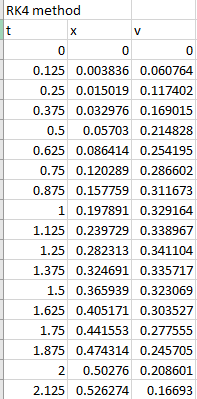
The first few solutions for displacement and velocity as a function of time for liner system is,

t x v
0 0 0
0.125 0.003836 0.060764
0.25 0.015019 0.117402
0.375 0.032976 0.169015
0.5 0.05703 0.214828
0.625 0.086414 0.254195
0.75 0.120289 0.286602
0.875 0.157759 0.311673
1 0.197891 0.329164
1.125 0.239729 0.338967
1.25 0.282313 0.341104
1.375 0.324691 0.335717
1.5 0.365939 0.323069
1.625 0.405171 0.303527
1.75 0.441553 0.277555
1.875 0.474314 0.245705
2 0.50276 0.208601
2.125 0.526274 0.16693
2.25 0.544332 0.121428
2.375 0.556503 0.072863
2.5 0.562454 0.02203
2.625 0.56195 -0.03027
2.75 0.554859 -0.08324
2.875 0.541146 -0.13608
3 0.520874 -0.18805
3.125 0.494199 -0.23842
3.25 0.461364 -0.28651
3.375 0.422694 -0.33168
3.5 0.378588 -0.37339
3.625 0.329513 -0.41112
3.75 0.275993 -0.44444
3.875 0.218601 -0.47301
4 0.157952 -0.49653
4.125 0.094688 -0.5148
4.25 0.029475 -0.52771
4.375 -0.03701 -0.53518
4.5 -0.1041 -0.53725
4.625 -0.1711 -0.53399
4.75 -0.23738 -0.52558
4.875 -0.30229 -0.51221
5 -0.36524 -0.49416

Explanation of Solution

Given Information:

The dynamic of a forced spring-mass-damper system is given as,

md2xdt2+cdxdt+k1x+k3x3=Pcos(ωt)

The values,

m=1 kgc=0.4 Ns/mP=0.5 Nω=0.5 /s

The initial condition, x=v=0.

Formula used:

The fourth-order RK method for dydt=f(t,y) is,

yn+1=yn+16(k1+2k2+2k3+k4)tn+1=tn+h

Where,

k1=hf(tn,yn)k2=hf(tn+h2,yn+k12)k3=hf(tn+h2,yn+k22)k4=hf(tn+h,yn+k3)

Calculation:

Consider the dynamic of a forced spring-mass-damper system,

md2xdt2+cdxdt+k1x+k3x3=Pcos(ωt)

As dxdt=v, replace dxdt by v in the above equation,

mdvdt+cv+k1x+k3x3=Pcos(ωt)

Divide both the sides of above equation by m,

dvdt=Pcos(ωt)mcvmk1xmk3x3m

Now, substitute the values m=1 kg, c=0.4 Ns/m, P=0.5 N and ω=0.5 /s in the above equation,

dvdt=0.5cos(0.5t)10.4v1k1x1k3x31dvdt=0.5cos(0.5t)0.4vk1xk3x3

For linear, substitute k1=1 and k3=0 in the equation,

dvdt=0.5cos(0.5t)0.4vx

Use VBA code for RK4 method as below to solve for x and v,

Code:

OptionExplicit

' Generate subfunction RK4SysTest()

Sub RK4SysTest()

'Declare the variables as integer

DimiAsInteger,m AsInteger,n AsInteger,j AsInteger

'Declare the variables as double

Dimx_iAsDouble,y_i(10)AsDouble,x_fAsDouble

DimdiffxAsDouble,x_outAsDouble

Dimx_p(200)AsDouble,y_p(200, 10)AsDouble

'Set the initial values

n =2

x_i=0

x_f=25

y_i(1)=0

y_i(2)=0

diffx=0.125

x_out=0.125

'move the values at a specific cell

Range("a3").Select

ActiveCell. Value="RK4 method"

'name each columns

ActiveCell. Offset(1, 0).Select

ActiveCell. Value="t"

ActiveCell. Offset(0, 1).Select

ActiveCell. Value="x"

ActiveCell. Offset(0, 1).Select

ActiveCell. Value="v"

' Call the function ODESolver

CallODESolver(x_i,y_i,x_f,diffx,x_out,x_p,y_p,m,n)

'Display the results in Sheet1

Sheets("Sheet1").Select

Range("a5:n205").ClearContents

Range("a5").Select

'Use for loop to store the different values of x_p

Fori=0To m

ActiveCell. Value=x_p(i)

'Use for loop to store the different values of y_p

For j =1To n

'Define the offset

ActiveCell. Offset(0, 1).Select

ActiveCell. Value=y_p(i,j)

Next j

'Define the offset

ActiveCell. Offset(1,-n).Select

Nexti

Range("a5").Select

EndSub

' Generate the subfunction ODESolver

SubODESolver(x_i,y_i,x_f,diffx,x_out,x_p,y_p,m,n)

'Declare the variables as integer

DimiAsInteger

'Declare the variables as double

Dim x AsDouble,y(10)AsDouble,x_endAsDouble

Dim h AsDouble

'Set the variables

m =0

'Store the value of x_i to x

x =x_i

'Use for loop to store the different values of y_i in y

Fori=1To n

y(i)=y_i(i)

Nexti

'Store the value of x in x_p

x_p(m)= x

'Use for loop to store the different values of y in y_p

Fori=1To n

y_p(m,i)= y(i)

Nexti

Do

'Display the result of x_end

x_end= x +x_out

If(x_end>x_f)Thenx_end=x_f

h =diffx

'Call the Integrator function

CallIntegrator(x,y,h,n,x_end)

m = m +1

'Store the value of x in x_p

x_p(m)= x

Fori=1To n

'Store the value of y in y_p

y_p(m,i)= y(i)

Nexti

'Use condition to exit the loop

If(x >=x_f)ThenExitDo

Loop

EndSub

' Generate a subfunction Integrator

SubIntegrator(x,y,h,n,x_end)

'Declare the variables

Dim j AsInteger

Dimynew(10)AsDouble

Do

'use loop for calculations

If(x_end- x < h)Then h =x_end- x

'Call the RK4Sys function

Call RK4Sys(x,y,h,n,ynew)

For j =1To n

'Store the different values of ynew to y

y(j)=ynew(j)

Next j

'Use condition to exit the loop

If(x >=x_end)ThenExitDo

Loop

EndSub

' Generate the subfunction RK4Sys

Sub RK4Sys(x,y,h,n,ynew)

'Declare the variables as integer

Dim j AsInteger

'Declare the variables as double

Dimy_m(10)AsDouble,y_e(10)AsDouble

Dim k_1(10)AsDouble,k_2(10)AsDouble,k_3(10)AsDouble,k_4(10)AsDouble

Dimslope(10)

'Call the Derivs function

CallDerivs(x,y,k_1)

For j =1To n

'Store the value of y(j) + k_1(j) * h / 2 in y_m

y_m(j)= y(j)+ k_1(j)* h /2

Next j

'Call the Derivs function

CallDerivs(x + h /2,y_m,k_2)

For j =1To n

'Store the value of y(j) + k_2(j) * h / 2 in y_m

y_m(j)= y(j)+ k_2(j)* h /2

Next j

'Call the Derivs function

CallDerivs(x + h /2,y_m,k_3)

For j =1To n

'Store the value of y(j) + k_3(j) * h in y_e

y_e(j)= y(j)+ k_3(j)* h

Next j

'Call the Derivs function

CallDerivs(x + h,y_e,k_4)

For j =1To n

'Store the value of k_1(j) + 2 * (k_2(j) + k_3(j)) + k_4(j)) / 6 in slope

slope(j)=(k_1(j)+2*(k_2(j)+ k_3(j))+ k_4(j))/6

Next j

For j =1To n

'Use formula to find ynew

ynew(j)= y(j)+ slope(j)* h

Next j

'Wrtite the next value of x

x = x + h

EndSub

' Generate the subfunction Derivs

SubDerivs(x,y,dydx)

'Write the ordinary differential equations

dydx(1)= y(2)

dydx(2)=-0.4* y(2)- y(1)+0.5* Cos(0.5* x)

EndSub

Output:

Package: Loose Leaf For Numerical Methods For Engineers With 1 Semester Connect Access Card, Chapter 28, Problem 49P , additional homework tip  1

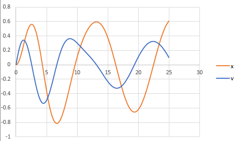
To draw the graph of the above results, follow the steps in excel sheet as given below,

Step 1: Select the cell from A4 to A205 and cell B4 to B205. Then, go to the Insert and select the scatter with smooth lines from the chart.

Step 2: Select the cell from A4 to A205 and cell C4 to C205. Then, go to the Insert and select the scatter with smooth lines from the chart.

Step 3: Select one of the graphs and paste it on another graph to merge the graphs.

The graph obtained is,
Package: Loose Leaf For Numerical Methods For Engineers With 1 Semester Connect Access Card, Chapter 28, Problem 49P , additional homework tip  2

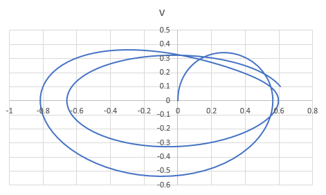
And, to draw the phase plane plot follow the steps as below,

Step 4: Select the column B and column C. Then, go to the Insert and select the scatter with smooth lines from the chart.

The graph obtained is,
Package: Loose Leaf For Numerical Methods For Engineers With 1 Semester Connect Access Card, Chapter 28, Problem 49P , additional homework tip  3

(b)

Expert Solution
Check Mark
To determine

To calculate: The displacement and velocity as a function of time for non-linear system where k1=1 and k3=0.5 if the dynamic of a forced spring-mass-damper system is given as md2xdt2+cdxdt+k1x+k3x3=Pcos(ωt).

Answer to Problem 49P

Solution:

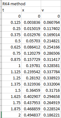
t x v
0 0 0
0.125 0.003836 0.060764
0.25 0.015019 0.117402
0.375 0.032976 0.169014
0.5 0.05703 0.214821
0.625 0.086412 0.254166
0.75 0.120279 0.286506
0.875 0.157729 0.311417
1 0.19781 0.328581
1.125 0.239542 0.337784
1.25 0.28192 0.338923
1.375 0.323936 0.332004
1.5 0.36459 0.31716
1.625 0.402907 0.294658
1.75 0.437953 0.264919
1.875 0.468859 0.228524
2 0.494837 0.186221
2.125 0.515205 0.138911
2.25 0.5294 0.087637
2.375 0.536996 0.033543
2.5 0.537718 -0.02217
2.625 0.531437 -0.07829
2.75 0.518177 -0.13366
2.875 0.498099 -0.18721
3 0.47149 -0.23801
3.125 0.438743 -0.28531
3.25 0.400333 -0.32852
3.375 0.3568 -0.36723
3.5 0.308725 -0.40117
3.625 0.256712 -0.43023
3.75 0.201374 -0.45436
3.875 0.143325 -0.47361
4 0.083172 -0.48804
4.125 0.021513 -0.49771
4.25 -0.04106 -0.50268
4.375 -0.10396 -0.50296
4.5 -0.1666 -0.49854
4.625 -0.2284 -0.48938
4.75 -0.28875 -0.47544
4.875 -0.34705 -0.45667
5 -0.40271 -0.43306

Explanation of Solution

Given Information:

The dynamic of a forced spring-mass-damper system is given as,

md2xdt2+cdxdt+k1x+k3x3=Pcos(ωt)

The values,

m=1 kgc=0.4 Ns/mP=0.5 Nω=0.5 /s

And,

k1=1 and k3=0.5

The initial condition, x=v=0.

Formula used:

The fourth-order RK method for dydt=f(t,y) is,

yn+1=yn+16(k1+2k2+2k3+k4)tn+1=tn+h

Where,

k1=hf(tn,yn)k2=hf(tn+h2,yn+k12)k3=hf(tn+h2,yn+k22)k4=hf(tn+h,yn+k3)

Calculation:

Consider the dynamic of a forced spring-mass-damper system,

md2xdt2+cdxdt+k1x+k3x3=Pcos(ωt)

As dxdt=v, replace dxdt by v in the above equation,

mdvdt+cv+k1x+k3x3=Pcos(ωt)

Divide both the sides of above equation by m,

dvdt=Pcos(ωt)mcvmk1xmk3x3m

Now, substitute the values m=1 kg, c=0.4 Ns/m, P=0.5 N and ω=0.5 /s in the above equation,

dvdt=0.5cos(0.5t)10.4v1k1x1k3x31dvdt=0.5cos(0.5t)0.4vk1xk3x3

For linear, substitute k1=1 and k3=0.5 in the equation,

dvdt=0.5cos(0.5t)0.4vx0.5x3

Use VBA code for RK4 method as below to solve for x and v,

Code:

OptionExplicit

' Generate subfunction RK4SysTest()

Sub RK4SysTest()

'Declare the variables as integer

DimiAsInteger,m AsInteger,n AsInteger,j AsInteger

'Declare the variables as double

Dimx_iAsDouble,y_i(10)AsDouble,x_fAsDouble

DimdiffxAsDouble,x_outAsDouble

Dimx_p(200)AsDouble,y_p(200, 10)AsDouble

'Set the initial values

n =2

x_i=0

x_f=25

y_i(1)=0

y_i(2)=0

diffx=0.125

x_out=0.125

'move the values at a specific cell

Range("a3").Select

ActiveCell. Value="RK4 method"

'name each columns

ActiveCell. Offset(1, 0).Select

ActiveCell. Value="t"

ActiveCell. Offset(0, 1).Select

ActiveCell. Value="x"

ActiveCell. Offset(0, 1).Select

ActiveCell. Value="v"

' Call the function ODESolver

CallODESolver(x_i,y_i,x_f,diffx,x_out,x_p,y_p,m,n)

'Display the results in Sheet1

Sheets("Sheet1").Select

Range("a5:n205").ClearContents

Range("a5").Select

'Use for loop to store the different values of x_p

Fori=0To m

ActiveCell. Value=x_p(i)

'Use for loop to store the different values of y_p

For j =1To n

'Define the offset

ActiveCell. Offset(0, 1).Select

ActiveCell. Value=y_p(i,j)

Next j

'Define the offset

ActiveCell. Offset(1,-n).Select

Nexti

Range("a5").Select

EndSub

' Generate the subfunction ODESolver

SubODESolver(x_i,y_i,x_f,diffx,x_out,x_p,y_p,m,n)

'Declare the variables as integer

DimiAsInteger

'Declare the variables as double

Dim x AsDouble,y(10)AsDouble,x_endAsDouble

Dim h AsDouble

'Set the variables

m =0

'Store the value of x_i to x

x =x_i

'Use for loop to store the different values of y_i in y

Fori=1To n

y(i)=y_i(i)

Nexti

'Store the value of x in x_p

x_p(m)= x

'Use for loop to store the different values of y in y_p

Fori=1To n

y_p(m,i)= y(i)

Nexti

Do

'Display the result of x_end

x_end= x +x_out

If(x_end>x_f)Thenx_end=x_f

h =diffx

'Call the Integrator function

CallIntegrator(x,y,h,n,x_end)

m = m +1

'Store the value of x in x_p

x_p(m)= x

Fori=1To n

'Store the value of y in y_p

y_p(m,i)= y(i)

Nexti

'Use condition to exit the loop

If(x >=x_f)ThenExitDo

Loop

EndSub

' Generate a subfunction Integrator

SubIntegrator(x,y,h,n,x_end)

'Declare the variables

Dim j AsInteger

Dimynew(10)AsDouble

Do

'use loop for calculations

If(x_end- x < h)Then h =x_end- x

'Call the RK4Sys function

Call RK4Sys(x,y,h,n,ynew)

For j =1To n

'Store the different values of ynew to y

y(j)=ynew(j)

Next j

'Use condition to exit the loop

If(x >=x_end)ThenExitDo

Loop

EndSub

' Generate the subfunction RK4Sys

Sub RK4Sys(x,y,h,n,ynew)

'Declare the variables as integer

Dim j AsInteger

'Declare the variables as double

Dimy_m(10)AsDouble,y_e(10)AsDouble

Dim k_1(10)AsDouble,k_2(10)AsDouble,k_3(10)AsDouble,k_4(10)AsDouble

Dimslope(10)

'Call the Derivs function

CallDerivs(x,y,k_1)

For j =1To n

'Store the value of y(j) + k_1(j) * h / 2 in y_m

y_m(j)= y(j)+ k_1(j)* h /2

Next j

'Call the Derivs function

CallDerivs(x + h /2,y_m,k_2)

For j =1To n

'Store the value of y(j) + k_2(j) * h / 2 in y_m

y_m(j)= y(j)+ k_2(j)* h /2

Next j

'Call the Derivs function

CallDerivs(x + h /2,y_m,k_3)

For j =1To n

'Store the value of y(j) + k_3(j) * h in y_e

y_e(j)= y(j)+ k_3(j)* h

Next j

'Call the Derivs function

CallDerivs(x + h,y_e,k_4)

For j =1To n

'Store the value of k_1(j) + 2 * (k_2(j) + k_3(j)) + k_4(j)) / 6 in slope

slope(j)=(k_1(j)+2*(k_2(j)+ k_3(j))+ k_4(j))/6

Next j

For j =1To n

'Use formula to find ynew

ynew(j)= y(j)+ slope(j)* h

Next j

'Wrtite the next value of x

x = x + h

EndSub

' Generate the subfunction Derivs

SubDerivs(x,y,dydx)

'Write the ordinary differential equations

dydx(1)= y(2)

dydx(2)=-0.4* y(2)- y(1)-0.5*(y(1))^3+0.5* Cos(0.5* x)

EndSub

Output:

Few data are shown below,

Package: Loose Leaf For Numerical Methods For Engineers With 1 Semester Connect Access Card, Chapter 28, Problem 49P , additional homework tip  4

To draw the graph of the above results, follow the steps in excel sheet as given below,

Step 1: Select the cell from A4 to A205 and cell B4 to B205. Then, go to the Insert and select the scatter with smooth lines from the chart.

Step 2: Select the cell from A4 to A205 and cell C4 to C205. Then, go to the Insert and select the scatter with smooth lines from the chart.

Step 3: Select one of the graphs and paste it on another graph to merge the graphs.

The graph obtained is,
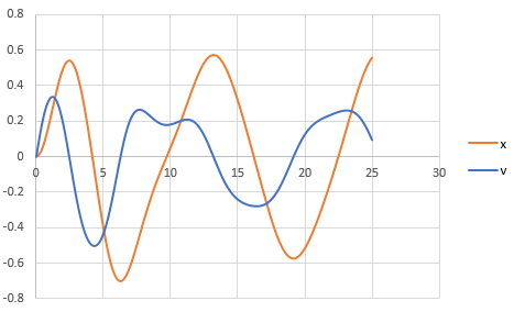
Package: Loose Leaf For Numerical Methods For Engineers With 1 Semester Connect Access Card, Chapter 28, Problem 49P , additional homework tip  5

And, to draw the phase plane plot follow the steps as below,

Step 4: Select the column B and column C. Then, go to the Insert and select the scatter with smooth lines from the chart.

The graph obtained is,
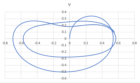
Package: Loose Leaf For Numerical Methods For Engineers With 1 Semester Connect Access Card, Chapter 28, Problem 49P , additional homework tip  6

Want to see more full solutions like this?

Subscribe now to access step-by-step solutions to millions of textbook problems written by subject matter experts!

Chapter 28 Solutions

Package: Loose Leaf For Numerical Methods For Engineers With 1 Semester Connect Access Card

Ch. 28 - An on is other malbatchre actor can be described...Ch. 28 - The following system is a classic example of stiff...Ch. 28 - 28.13 A biofilm with a thickness grows on the...Ch. 28 - 28.14 The following differential equation...Ch. 28 - Prob. 15PCh. 28 - 28.16 Bacteria growing in a batch reactor utilize...Ch. 28 - 28.17 Perform the same computation for the...Ch. 28 - Perform the same computation for the Lorenz...Ch. 28 - The following equation can be used to model the...Ch. 28 - Perform the same computation as in Prob. 28.19,...Ch. 28 - 28.21 An environmental engineer is interested in...Ch. 28 - 28.22 Population-growth dynamics are important in...Ch. 28 - 28.23 Although the model in Prob. 28.22 works...Ch. 28 - 28.25 A cable is hanging from two supports at A...Ch. 28 - 28.26 The basic differential equation of the...Ch. 28 - 28.27 The basic differential equation of the...Ch. 28 - A pond drains through a pipe, as shown in Fig....Ch. 28 - 28.29 Engineers and scientists use mass-spring...Ch. 28 - Under a number of simplifying assumptions, the...Ch. 28 - 28.31 In Prob. 28.30, a linearized groundwater...Ch. 28 - The Lotka-Volterra equations described in Sec....Ch. 28 - The growth of floating, unicellular algae below a...Ch. 28 - 28.34 The following ODEs have been proposed as a...Ch. 28 - 28.35 Perform the same computation as in the first...Ch. 28 - Solve the ODE in the first part of Sec. 8.3 from...Ch. 28 - 28.37 For a simple RL circuit, Kirchhoff’s voltage...Ch. 28 - In contrast to Prob. 28.37, real resistors may not...Ch. 28 - 28.39 Develop an eigenvalue problem for an LC...Ch. 28 - 28.40 Just as Fourier’s law and the heat balance...Ch. 28 - 28.41 Perform the same computation as in Sec....Ch. 28 - 28.42 The rate of cooling of a body can be...Ch. 28 - The rate of heat flow (conduction) between two...Ch. 28 - Repeat the falling parachutist problem (Example...Ch. 28 - 28.45 Suppose that, after falling for 13 s, the...Ch. 28 - 28.46 The following ordinary differential equation...Ch. 28 - 28.47 A forced damped spring-mass system (Fig....Ch. 28 - 28.48 The temperature distribution in a tapered...Ch. 28 - 28.49 The dynamics of a forced spring-mass-damper...Ch. 28 - The differential equation for the velocity of a...Ch. 28 - 28.51 Two masses are attached to a wall by linear...
Knowledge Booster
Background pattern image
Advanced Math
Learn more about
Need a deep-dive on the concept behind this application? Look no further. Learn more about this topic, advanced-math and related others by exploring similar questions and additional content below.
Recommended textbooks for you
Text book image
Advanced Engineering Mathematics
Advanced Math
ISBN:9780470458365
Author:Erwin Kreyszig
Publisher:Wiley, John & Sons, Incorporated
Text book image
Numerical Methods for Engineers
Advanced Math
ISBN:9780073397924
Author:Steven C. Chapra Dr., Raymond P. Canale
Publisher:McGraw-Hill Education
Text book image
Introductory Mathematics for Engineering Applicat...
Advanced Math
ISBN:9781118141809
Author:Nathan Klingbeil
Publisher:WILEY
Text book image
Mathematics For Machine Technology
Advanced Math
ISBN:9781337798310
Author:Peterson, John.
Publisher:Cengage Learning,
Text book image
Basic Technical Mathematics
Advanced Math
ISBN:9780134437705
Author:Washington
Publisher:PEARSON
Text book image
Topology
Advanced Math
ISBN:9780134689517
Author:Munkres, James R.
Publisher:Pearson,
Chain Rule dy:dx = dy:du*du:dx; Author: Robert Cappetta;https://www.youtube.com/watch?v=IUYniALwbHs;License: Standard YouTube License, CC-BY
CHAIN RULE Part 1; Author: Btech Maths Hub;https://www.youtube.com/watch?v=TIAw6AJ_5Po;License: Standard YouTube License, CC-BY