
Concept explainers
Videos
The following equations define the concentrations of threereactants:
If the initial conditions are
To calculate: The concentration for the times from
Initials conditions are
Answer to Problem 7P
Solution:
The concentration of the reactants
The concentration of the reactants
The concentration of the reactants
The concentration of the reactants
Explanation of Solution
Given information:
The system of equations,
Initial conditions,
Formula used:
To calculate the values of
Eigen value
Calculation:
Consider the system of first order nonlinear differential equation of reactants
To calculate equilibrium points, consider the equations given below:
Compare the system of first order nonlinear differential equations with the above equations,
Therefore, the equilibrium point is,
Suppose, the system of non-linear differential equations are equal to some functions, that is,
Now, compare these equations with system of non-linear differential equations,
Now, find the Jacobian matrix,
Then, the Jacobian matrix at the equilibrium points
Now, the linearized system corresponding to nonlinear system of differential equation is,
Let,
Suppose,
Thus,
Now calculate the determinant as,
Therefore, the eigenvalues of the matrix are
Now, find the eigenvector corresponding to each eigenvalue of the matrix.
The eigenvector is,
Where,
Substitute the value of X in
Put
Put
Put
Therefore, the eigenvector corresponding to each eigenvalue of the matrix are respectively
Hence, the solution of the system of nonlinear differential equation is,
After solve the above equation,
Then the values of
The initial conditionsgiven as,
Now, apply the initial condition in the above equations,
This imply that,
Then,
Substitute, the value of
The concentration at
Therefore, theconcentration of the reactants
Now, the concentration at
Therefore, the concentration of the reactants
Now, the concentration at
Therefore, the concentration of the reactants
Now, the concentration at
Use the following MATLAB code to plot the concentrationvalues,
Execute the above to obtain the plot as,
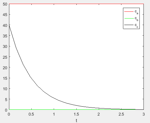
Therefore, the concentration of the reactants
Hence, the concentration of the reactants
Want to see more full solutions like this?
Chapter 28 Solutions
Numerical Methods for Engineers


- Find the intensities of earthquakes whose magnitudes are (a) R=6.0 and (b) R=7.9.arrow_forwardTsunami Waves and BreakwatersThis is a continuation of Exercise 16. Breakwaters affect wave height by reducing energy. See Figure 5.30. If a tsunami wave of height H in a channel of width W encounters a breakwater that narrows the channel to a width w, then the height h of the wave beyond the breakwater is given by h=HR0.5, where R is the width ratio R=w/W. a. Suppose a wave of height 8 feet in a channel of width 5000feet encounters a breakwater that narrows the channel to 3000feet. What is the height of the wave beyond the breakwater? b. If a channel width is cut in half by a breakwater, what is the effect on wave height? 16. Height of Tsunami WavesWhen waves generated by tsunamis approach shore, the height of the waves generally increases. Understanding the factors that contribute to this increase can aid in controlling potential damage to areas at risk. Greens law tells how water depth affects the height of a tsunami wave. If a tsunami wave has height H at an ocean depth D, and the wave travels to a location with water depth d, then the new height h of the wave is given by h=HR0.25, where R is the water depth ratio given by R=D/d. a. Calculate the height of a tsunami wave in water 25feet deep if its height is 3feet at its point of origin in water 15,000feet deep. b. If water depth decreases by half, the depth ratio R is doubled. How is the height of the tsunami wave affected?arrow_forward
 Algebra and Trigonometry (MindTap Course List)AlgebraISBN:9781305071742Author:James Stewart, Lothar Redlin, Saleem WatsonPublisher:Cengage Learning
 College AlgebraAlgebraISBN:9781305115545Author:James Stewart, Lothar Redlin, Saleem WatsonPublisher:Cengage Learning
 College Algebra (MindTap Course List)AlgebraISBN:9781305652231Author:R. David Gustafson, Jeff HughesPublisher:Cengage Learning
 Algebra: Structure And Method, Book 1AlgebraISBN:9780395977224Author:Richard G. Brown, Mary P. Dolciani, Robert H. Sorgenfrey, William L. ColePublisher:McDougal Littell
 Functions and Change: A Modeling Approach to Coll...AlgebraISBN:9781337111348Author:Bruce Crauder, Benny Evans, Alan NoellPublisher:Cengage Learning