
Concept explainers
Videos
The basic differential equation of the elastic curve for a uniformly loaded beam (Fig. P28.27) is given as
Where
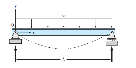
FIGURE P28.27
(a)
To calculate: The deflection of the beam by the finite-difference method with
Answer to Problem 27P
Solution:
The deflection of the beam by the finite-difference method is,
| x | y | y-Analytical |
| 0 | 0 | 0 |
| 24 | ||
| 48 | ||
| 72 | ||
| 96 | ||
| 120 | 0 | 0 |
Explanation of Solution
Given Information:
The differential equation for the elastic curve for a uniformly loaded beam is given as,
Formula to find analytical value,
Where,
The modulus of elasticity,
The moment of inertia,
The values,
Formula used:
The conversion formula,
The value of second order derivative by finite difference method is given as,
Calculation:
Consider the equation,
Rewrite the above equation as,
Substitute the values,
Now, the second order derivative by finite difference method gives,
Therefore,
Put
The boundary condition is,
Put
Substitute
Put
Substitute
Put
Substitute
The matrix form of the above equations is given as below,
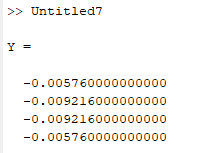
Use MATLAB to find the solution of the above system as below,
Code:
%Write the matrix
A=[-2 1 0 0; 1 -2 1 0; 0 1 -2 1; 0 0 1 -2];
%write the values of rhs
b=[0.002304 0.003456 0.003456 0.002304]';
%find the result
Y=A\b
Output:
Now, for the analytical value, consider the equation
Substitute the values,
Use excel to find the values of y at different values of x as below,
Step 1: Name the column A as x and go to column A2 and put 0 then go to column A3 and write the formula as,
=A2+24
Then, Press enter and drag the column up to
Step 2: Now name the column B as y and go to column B2 andwrite the formula as,
=2.89236*10^(-10)*A2*(120*A2^2-0.5*A2^3-864000)
Step 3: Press enter and drag the column up to
The result obtained as,
| x | y-Analytical |
| 0 | 0 |
| 24 | |
| 48 | |
| 72 | |
| 96 | |
| 120 | 0 |
(b)
To calculate: The deflection of the beam by the shooting method with
Answer to Problem 27P
Solution:
A few values of deflection of the beam by the shooting method is,
| x | y | z |
| 0 | 0 | -1.6E-06 |
| 0.25 | -4.1E-07 | -1.6E-06 |
| 0.5 | -8.2E-07 | -1.6E-06 |
| 0.75 | -1.2E-06 | -1.6E-06 |
| 1 | -1.6E-06 | -1.6E-06 |
| 1.25 | -2E-06 | -1.5E-06 |
| 1.5 | -2.4E-06 | -1.4E-06 |
| 1.75 | -2.8E-06 | -1.4E-06 |
| 2 | -3.2E-06 | -1.3E-06 |
| 2.25 | -3.5E-06 | -1.2E-06 |
| 2.5 | -3.8E-06 | -1.1E-06 |
| 2.75 | -4.1E-06 | -1E-06 |
| 3 | -4.4E-06 | -9E-07 |
Explanation of Solution
Given Information:
The differential equation for the elastic curve for a uniformly loaded beam is given as,
Formula to find analytical value,
Where,
The modulus of elasticity,
The moment of inertia,
The values,
Formula used:
The conversion formula,
Calculation:
Consider the equation,
Rewrite the equation as,
Assume
Substitute the values,
Use VBA program as below to solve the above differential equation as below,
Code:
OptionExplicit
'Create a function find
Subfind()
'declare the variables as integer
Dim n AsInteger, j AsInteger
'declare the variables as double
DimdydxAsDouble, x AsDouble, dy2dx AsDouble, yanalAsDouble, E AsDouble, I AsDouble, w AsDouble, L AsDouble
DimolddydxAsDouble, oldy AsDouble, y AsDouble, h AsDouble
'Set the values of the variables
E =30000
I =800
w =1
L =10
y =0
x =0
h =0.25
dydx=0
'store dydx and analytical solution
dydx= caldydx(w, E, I, L, x)
yanal= caly(w, E, I, L, x)
'use for loop to determine different value of y and y analytical
For j =1 To41
'store the value of y at oldy and dydx in olddydx
oldy = y
olddydx= dydx
'Store d2ydx, dydx and analytical solution
dy2dx = caldy2dx(w, E, I, L, x)
dydx= caldydx(w, E, I, L, x)
yanal= caly(w, E, I, L, x)
'move to the cell b3
Range("b1"). Select
ActiveCell.Value="shooting method"
'Assign name to the columns
ActiveCell.Offset(1,0). Select
ActiveCell.Value="x"
ActiveCell.Offset(0,1). Select
ActiveCell.Value="y"
ActiveCell.Offset(0,1). Select
ActiveCell.Value="z"
ActiveCell.Offset(0,1). Select
ActiveCell.Value="dy2dx"
ActiveCell.Offset(0,1). Select
ActiveCell.Value="y-anal"
'dislay values in cell
Range("b2"). Select
ActiveCell.Offset(j,0). Select
ActiveCell.Value= x
ActiveCell.Offset(0,1). Select
ActiveCell.Value= oldy
ActiveCell.Offset(0,1). Select
ActiveCell.Value= dydx
ActiveCell.Offset(0,1). Select
ActiveCell.Value= dy2dx
ActiveCell.Offset(0,1). Select
ActiveCell.Value= yanal
'Write the next value of x
x = x + h
'Write the next value of y by euler method
y = oldy + olddydx* h
Next
EndSub
'Define d2ydx function
Function caldy2dx(w, E, I, L, x)
'Declare the variables
Dim t AsDouble
'Write the formula
t =((w * L * x)/(2* E * I))-((w * x * x)/(2* E * I))
'Store the value
caldy2dx = t
EndFunction
'Define dydx
Functioncaldydx(w, E, I, L, x)
'Declare the variables
Dim t AsDouble, c AsDouble
'Set the values
c =-0.000001648
'Write the formula
t =((w * L * x * x)/(4* E * I))-((w * x * x * x)/(6* E * I))+ c
'Store the value
caldydx= t
EndFunction
'Define the function caly for analytical value
Functioncaly(w, E, I, L, x)
'Declare the variables
Dim t AsDouble
'Write the formula
t =((w * L * x * x * x)/(12* E * I))-((w * x * x * x * x)/(24* E * I))-((w * L * L * L * x)/(24* E * I))
'Store the value
caly= t
EndFunction
Output:
| shooting method | ||||
| x | y | z | dy2dx | y-anal |
| 0 | 0 | -1.6E-06 | 0 | 0 |
| 0.25 | -4.1E-07 | -1.6E-06 | 5.08E-08 | -4.3E-07 |
| 0.5 | -8.2E-07 | -1.6E-06 | 9.9E-08 | -8.6E-07 |
| 0.75 | -1.2E-06 | -1.6E-06 | 1.45E-07 | -1.3E-06 |
| 1 | -1.6E-06 | -1.6E-06 | 1.88E-07 | -1.7E-06 |
| 1.25 | -2E-06 | -1.5E-06 | 2.28E-07 | -2.1E-06 |
| 1.5 | -2.4E-06 | -1.4E-06 | 2.66E-07 | -2.5E-06 |
| 1.75 | -2.8E-06 | -1.4E-06 | 3.01E-07 | -2.9E-06 |
| 2 | -3.2E-06 | -1.3E-06 | 3.33E-07 | -3.2E-06 |
| 2.25 | -3.5E-06 | -1.2E-06 | 3.63E-07 | -3.6E-06 |
| 2.5 | -3.8E-06 | -1.1E-06 | 3.91E-07 | -3.9E-06 |
| 2.75 | -4.1E-06 | -1E-06 | 4.15E-07 | -4.2E-06 |
| 3 | -4.4E-06 | -9E-07 | 4.38E-07 | -4.4E-06 |
| 3.25 | -4.7E-06 | -7.9E-07 | 4.57E-07 | -4.6E-06 |
| 3.5 | -4.9E-06 | -6.7E-07 | 4.74E-07 | -4.8E-06 |
| 3.75 | -5.1E-06 | -5.5E-07 | 4.88E-07 | -5E-06 |
| 4 | -5.2E-06 | -4.3E-07 | 5E-07 | -5.2E-06 |
| 4.25 | -5.4E-06 | -3E-07 | 5.09E-07 | -5.3E-06 |
| 4.5 | -5.5E-06 | -1.7E-07 | 5.16E-07 | -5.4E-06 |
| 4.75 | -5.6E-06 | -4.2E-08 | 5.2E-07 | -5.4E-06 |
| 5 | -5.6E-06 | 8.81E-08 | 5.21E-07 | -5.4E-06 |
| 5.25 | -5.6E-06 | 2.18E-07 | 5.2E-07 | -5.4E-06 |
| 5.5 | -5.6E-06 | 3.48E-07 | 5.16E-07 | -5.4E-06 |
| 5.75 | -5.5E-06 | 4.76E-07 | 5.09E-07 | -5.3E-06 |
| 6 | -5.4E-06 | 6.02E-07 | 5E-07 | -5.2E-06 |
| 6.25 | -5.3E-06 | 7.26E-07 | 4.88E-07 | -5E-06 |
| 6.5 | -5.2E-06 | 8.46E-07 | 4.74E-07 | -4.8E-06 |
| 6.75 | -5E-06 | 9.62E-07 | 4.57E-07 | -4.6E-06 |
| 7 | -4.8E-06 | 1.07E-06 | 4.38E-07 | -4.4E-06 |
| 7.25 | -4.5E-06 | 1.18E-06 | 4.15E-07 | -4.2E-06 |
| 7.5 | -4.3E-06 | 1.28E-06 | 3.91E-07 | -3.9E-06 |
| 7.75 | -4E-06 | 1.38E-06 | 3.63E-07 | -3.6E-06 |
| 8 | -3.7E-06 | 1.46E-06 | 3.33E-07 | -3.2E-06 |
| 8.25 | -3.3E-06 | 1.54E-06 | 3.01E-07 | -2.9E-06 |
| 8.5 | -3E-06 | 1.61E-06 | 2.66E-07 | -2.5E-06 |
| 8.75 | -2.6E-06 | 1.68E-06 | 2.28E-07 | -2.1E-06 |
| 9 | -2.2E-06 | 1.73E-06 | 1.88E-07 | -1.7E-06 |
| 9.25 | -1.7E-06 | 1.77E-06 | 1.45E-07 | -1.3E-06 |
| 9.5 | -1.3E-06 | 1.8E-06 | 9.9E-08 | -8.6E-07 |
| 9.75 | -8.7E-07 | 1.82E-06 | 5.08E-08 | -4.3E-07 |
| 10 | -4.2E-07 | 1.82E-06 | 0 | 0 |
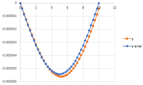
Now, to draw the graph of y and y-analytical follow the step as below,
Step 1: Select the cell from B2 to B43 and cell C2 to C43. Then, go to the Insert and select the scatter with smooth lines from the chart.
Step 2: Select the cell from B2 to B43 and cell F2 to F43. Then, go to the Insert and select the scatter with smooth lines from the chart.
Step 3: Select one of the graphs and paste it on another graph to merge the graphs.
The graph obtained is,
Want to see more full solutions like this?
Chapter 28 Solutions
Numerical Methods for Engineers
Additional Math Textbook Solutions
Fundamentals of Differential Equations (9th Edition)
Advanced Engineering Mathematics
Basic Technical Mathematics


 Advanced Engineering MathematicsAdvanced MathISBN:9780470458365Author:Erwin KreyszigPublisher:Wiley, John & Sons, Incorporated
 Numerical Methods for EngineersAdvanced MathISBN:9780073397924Author:Steven C. Chapra Dr., Raymond P. CanalePublisher:McGraw-Hill Education
 Introductory Mathematics for Engineering Applicat...Advanced MathISBN:9781118141809Author:Nathan KlingbeilPublisher:WILEY
 Mathematics For Machine TechnologyAdvanced MathISBN:9781337798310Author:Peterson, John.Publisher:Cengage Learning,
