
Concept explainers
Videos
a.
Find the median household income for 2013.
a.
Answer to Problem 68SE
The median household income for 2013 is $52,100.
Explanation of Solution
Calculation:
The data represent the sample of 14 household incomes for 2013. It is also known that the median annual household income for 2007 was $55,500.
The variable “household income” is stored in the column “C1” in the MINITAB worksheet.
Median:
Software Procedure:
Step-by-step procedure to obtain the median using MINITAB software:
- Choose Stat > Basic Statistics > Display
Descriptive Statistics . - In Variables enter the columns C1.
- In Statistics select median.
- Click OK.
The output obtained using MINITAB software is given below:
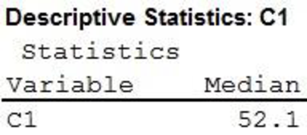
Thus, the median household income for 2013 is $52,100.
b.
Find the percentage change in the median household income from 2007 to 2013.
b.
Answer to Problem 68SE
The percentage change in the median household income from 2007 to 2013 is –6.1%.
Explanation of Solution
Calculation:
The median household income in 2007 is $55,500 (55.5). From Part (a), it can be seen that the median household income in 2013 is $52,100.
The percentage change in the median household income from 2007 to 2013 can be obtained as follows:
Thus, the percentage change in the median household income from 2007 to 2013 is –6.1%.
Therefore, there is 6.1% decrease in the median household income from 2007 to 2013.
c.
Find the first and third
c.
Answer to Problem 68SE
The first and third quartiles are $50,750 and $52,600, respectively.
Explanation of Solution
Calculation:
First quartile and Third quartile:
Software Procedure:
Step-by-step procedure to obtain the first and third quartiles using MINITAB software:
- Choose Stat > Basic Statistics >Display Descriptive Statistics.
- Click OK.
- In Variables, enter the column of C1.
- In Statistics select First quartile and Third quartile.
- Click OK.
The output obtained using MINITAB software is given below:
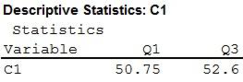
Therefore, the first and third quartiles are $50,750 and $52,600, respectively.
d.
Find the
d.
Answer to Problem 68SE
The five-number summary is as follows:
- Minimum: $46,500,
- First quartile: $50,750,
- Median: $52,100,
- Third quartile: $52,600,
- Maximum: $64,500.
Explanation of Solution
Calculation:
Five-number summary: Minimum, Q1, median, Q3, and maximum.
Five-number summary:
Software Procedure:
Step-by-step procedure to obtain the five-number summary using MINITAB software:
- Choose Stat > Basic Statistics >Display Descriptive Statistics.
- Click OK.
- In Variables, enter the column of C1.
- In Statistics, select Minimum, First quartile, Median, Third quartile and Maximum.
- Click OK.
The output obtained using MINITAB software is given below:
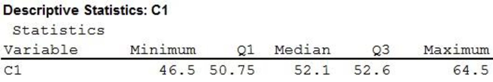
Thus, the five-number summary for data has been obtained.
e.
Identify the outliers using the z-score approach.
Check whether the approach that uses the values of the first and third quartiles and the
e.
Answer to Problem 68SE
The outlier obtained using the z-score approach is $64,500.
No, the approach that uses the values of the first and third quartiles and the interquartile
Explanation of Solution
Calculation:
The z-score:
where
Mean and Standard deviation:
Software Procedure:
Step-by-step procedure to obtain the mean and standard deviation using MINITAB software:
- Choose Stat > Basic Statistics > Display Descriptive Statistics.
- Click OK.
- In Variables, enter the column of C1.
- In Statistics select Mean and Standard deviation.
- Click OK.
The output obtained using MINITAB software is given below:
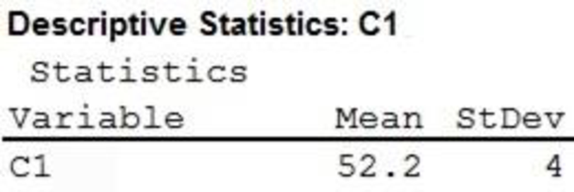
From the MINITAB output, it is clear that the mean and standard deviation are 52.2 and 4, respectively.
The z-score corresponding to 49.4 can be obtained as follows:
Substitute
Thus, the z-score corresponding to 49.4 is –0.70.
Similarly, the z-scores corresponding to other values can be obtained as follows:
| Values | z-score |
| 46.5 | –1.42 |
| 48.7 | –0.87 |
| 49.4 | –0.70 |
| 51.2 | –0.25 |
| 51.3 | –0.22 |
| 51.6 | –0.15 |
| 52.1 | –0.02 |
| 52.1 | –0.02 |
| 52.2 | 0.00 |
| 52.4 | 0.05 |
| 52.5 | 0.07 |
| 52.9 | 0.17 |
| 53.4 | 0.30 |
| 64.5 | 3.07 |
Outlier detection using the 3 standard deviation distance criterion:
An observation is considered as a potential outlier if the absolute value of the z-score of the observation is greater than 3, that is, if the observation lies more than 3 standard deviations away (above or below) from the mean value.
From the table, it can be seen that the z-score corresponding to 64.5 is greater than 3. Thus, the observation of 64.5 is considered to be an outlier.
Interquartile range (IQR):
- The outliers in the data set can be obtained as shown below:
By substituting the corresponding values, we obtain the following results:
A value in the dataset is said to be an outlier if it falls outside the interval from 47.98 to 55.375. In general, the data values less than 47.98 or greater than 55.375 are considered as the outliers.
The first observation (46.5) is less than 47.98, and the observation (64.5) is greater than 55.375. Hence, there are two outliers, $49,400 and $64,500.
Thus, the results obtained in two approaches are not the same.
Want to see more full solutions like this?
Chapter 3 Solutions
MindTap Business Statistics, 1 term (6 months) Printed Access Card for Anderson/Sweeney/Williams/Camm/Cochran's Essentials of Statistics for Business and Economics, 8th


 MATLAB: An Introduction with ApplicationsStatisticsISBN:9781119256830Author:Amos GilatPublisher:John Wiley & Sons Inc
 Probability and Statistics for Engineering and th...StatisticsISBN:9781305251809Author:Jay L. DevorePublisher:Cengage Learning
 Statistics for The Behavioral Sciences (MindTap C...StatisticsISBN:9781305504912Author:Frederick J Gravetter, Larry B. WallnauPublisher:Cengage Learning
 Elementary Statistics: Picturing the World (7th E...StatisticsISBN:9780134683416Author:Ron Larson, Betsy FarberPublisher:PEARSON
 The Basic Practice of StatisticsStatisticsISBN:9781319042578Author:David S. Moore, William I. Notz, Michael A. FlignerPublisher:W. H. Freeman
 Introduction to the Practice of StatisticsStatisticsISBN:9781319013387Author:David S. Moore, George P. McCabe, Bruce A. CraigPublisher:W. H. Freeman