Control Systems Engineering
7th Edition
ISBN: 9781118170519
Author: Norman S. Nise
Publisher: WILEY
expand_more
expand_more
format_list_bulleted
Concept explainers
Videos
Textbook Question
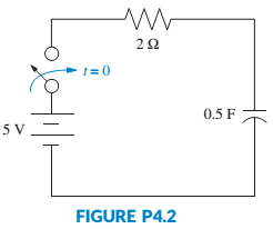
Chapter 4, Problem 4P
Find the capacitor voltage in the network shown in Figure P4.2 if the switch closes at t = 0. Assume zero initial conditions. Also find the time constant, rise time, and settling time for the capacitor voltage.
[Sections: 4.2, 4.3]
Expert Solution & Answer
Want to see the full answer?
Check out a sample textbook solution
Students have asked these similar questions
Represent the translational mechanical system shown in state space, where x3(t) is the output.
Find the state-space equation of the following mass-springdamper system. Assume that the bottom surface is frictionless. The input is external forcef(t)and the output is displacementx1(t)
Find the transfer function, G(s) = X3(s)/F(s), for the translational mechanical system shown in Figure P2.13.
Step-by-step procedure is highly appreciated.
Chapter 4 Solutions
Control Systems Engineering
Ch. 4 - Prob. 1RQCh. 4 - What does the performance specification for a...Ch. 4 - Prob. 3RQCh. 4 - In a system with an input and an output, what...Ch. 4 - Prob. 5RQCh. 4 - Prob. 6RQCh. 4 - 7. What is the difference between the natural...Ch. 4 - Prob. 8RQCh. 4 - Prob. 9RQCh. 4 - Prob. 10RQ
Ch. 4 - List five specifications for a second-order...Ch. 4 - Prob. 12RQCh. 4 - What pole locations characterize (1) the...Ch. 4 - Prob. 14RQCh. 4 - How can you justify pole-zero cancellation?Ch. 4 - Prob. 16RQCh. 4 - 17. What is the relationship between , which...Ch. 4 - Name a major advantage of using time-domain...Ch. 4 - Prob. 19RQCh. 4 - What three pieces of information must be given in...Ch. 4 - 21. How can the poles of a system be found from...Ch. 4 - Prob. 1PCh. 4 - Prob. 2PCh. 4 - MATIAB ML 3. Plot the step responses for Problem 2...Ch. 4 - Find the capacitor voltage in the network shown in...Ch. 4 - For the system shown in Figure P4.3, (a) find an...Ch. 4 - Prob. 8PCh. 4 - MATLAB ML 9. Use MATLAB to find the poles of...Ch. 4 - Find the transfer function and poles of the system...Ch. 4 - MATLAB ML 11. Repeat Problem 10 using MATLAB....Ch. 4 - Write the general form of the capacitor voltage...Ch. 4 - Solve for x(t) in the system shown in Figure P4.5...Ch. 4 - Prob. 15PCh. 4 - Prob. 16PCh. 4 - Calculate the exact response of each system of...Ch. 4 - Prob. 18PCh. 4 - Prob. 19PCh. 4 - For each of the second-order systems that follow,...Ch. 4 - MATLAB ML 21. Repeat Problem 20 using MATLAB. Have...Ch. 4 - GUI Tool GUIT
22. Use MATLAB’s LTI Viewer and...Ch. 4 - Prob. 23PCh. 4 - Find the transfer function of a second-order...Ch. 4 - For the system shown in Figure P4.7, do the...Ch. 4 - For the system shown in Figure P4.8, a step torque...Ch. 4 - Prob. 28PCh. 4 - Prob. 29PCh. 4 - Prob. 30PCh. 4 - Prob. 31PCh. 4 - Prob. 32PCh. 4 - Prob. 33PCh. 4 - Prob. 34PCh. 4 - Prob. 35PCh. 4 - Prob. 36PCh. 4 - State Space SS 38. A system is represented by the...Ch. 4 - Prob. 39PCh. 4 - Prob. 40PCh. 4 - State Space SS 41. Given the following system...Ch. 4 - State Space SS 42. Solve the following state...Ch. 4 - Prob. 43PCh. 4 - Prob. 44PCh. 4 - Prob. 46PCh. 4 - Prob. 47PCh. 4 - Prob. 48PCh. 4 - Prob. 53PCh. 4 - Prob. 54PCh. 4 - A MOEMS (optical MEMS) is a MEMS (Micro...Ch. 4 - Prob. 56PCh. 4 - Prob. 59PCh. 4 - Prob. 60PCh. 4 - Prob. 61PCh. 4 - Prob. 63PCh. 4 - Prob. 67PCh. 4 - Figure P4.l6 shows the step response of an...Ch. 4 - Figure P4. I 7 shows the free-body diagrams for...Ch. 4 - Find an equation that relates 2% settling time to...Ch. 4 - Prob. 74PCh. 4 - Prob. 75PCh. 4 - 76. Find J and K in the rotational system shown in...Ch. 4 - Given the system shown in Figure P4.22, find the...Ch. 4 - Prob. 78PCh. 4 - Find M and K, shown in the system of Figure P4.24,...Ch. 4 - If vi(t) is a step voltage in the network shown in...Ch. 4 - Prob. 81PCh. 4 - Prob. 82PCh. 4 - For the circuit shown in Figure P4.26, find the...Ch. 4 - Prob. 84PCh. 4 - Prob. 86P
Knowledge Booster


Learn more about
Need a deep-dive on the concept behind this application? Look no further. Learn more about this topic, mechanical-engineering and related others by exploring similar questions and additional content below.Similar questions
- Obtain the state space model of the system shown below. Use equations for control theory state space modeling.arrow_forwardFind the transfer function,G(s)=Z1(s)/H(s) Find the state space model.arrow_forwardFind a state space representation for the network shown below when the output is the displacement at M3.arrow_forward
- Get the input-output model Get the Transfer Function Get representation in State Variablesarrow_forwardSketch the level response for a bathtub with cross-sectional area of 8 ft 2 as a function of time for the following sequence of events; assume an initial level of 0.5 ft with the drain open. The inflow and outflow are initially equal to2ft3/min.(a)The drain is suddenly closed, and the inflow remains con-stant for 3 min (0≤t≤3).(b)The drain is opened for 15 min; assume a time constant in a linear transfer function of 3 min, so a steady state is essentially reached (3≤t≤18) (c)The inflow rate is doubled for 6 min (18≤t≤24).(d)The inflow rate is returned to its original value for 16 min(24≤t≤40).arrow_forwardDerive the state-space representation of the following system where the input is f(t) and the outputs isthe y1 =X1, y2=X2, y3=X3arrow_forward
- Reduce the block diagram shown in Figure below to a single transfer function, T(s) = C(s)/R(s) Use the block diagram reduction method.arrow_forwardMATLAB PROBLEMarrow_forwardA velocity of a vehicle is required to be controlled and maintained constant even if there are disturbances because of wind, or road surface variations. The forces that are applied on the vehicle are the engine force (u), damping/resistive force (b*v) that opposing the motion, and inertial force (m*a). A simplified model is shown in the free body diagram below. From the free body diagram, the ordinary differential equation of the vehicle is: m * dv(t)/ dt + bv(t) = u (t) Where: v (m/s) is the velocity of the vehicle, b [Ns/m] is the damping coefficient, m [kg] is the vehicle mass, u [N] is the engine force. Question: Assume that the vehicle initially starts from zero velocity and zero acceleration. Then, (Note that the velocity (v) is the output and the force (w) is the input to the system): 1. What is the order of this system?arrow_forward
- A velocity of a vehicle is required to be controlled and maintained constant even if there are disturbances because of wind, or road surface variations. The forces that are applied on the vehicle are the engine force (u), damping/resistive force (b*v) that opposing the motion, and inertial force (m*a). A simplified model is shown in the free body diagram below. From the free body diagram, the ordinary differential equation of the vehicle is: m * dv(t)/ dt + bv(t) = u (t) Where: v (m/s) is the velocity of the vehicle, b [Ns/m] is the damping coefficient, m [kg] is the vehicle mass, u [N] is the engine force. Question: Assume that the vehicle initially starts from zero velocity and zero acceleration. Then, (Note that the velocity (v) is the output and the force (w) is the input to the system): A. Use Laplace transform of the differential equation to determine the transfer function of the system.arrow_forwardFor the system shown in the figure; the input is the torque T and the outputs are the displacements Q1 and Q2.a) Draw the free body diagrams and derive the equations of motions. (Assume Q1 >Q 2).b) Obtain the state-space representation by using the given state variables (vector)arrow_forwardThe ratio of output to input of a system in Laplace domain is known as Transfer function . Select one: True Falsearrow_forward
arrow_back_ios
SEE MORE QUESTIONS
arrow_forward_ios
Recommended textbooks for you
 Elements Of ElectromagneticsMechanical EngineeringISBN:9780190698614Author:Sadiku, Matthew N. O.Publisher:Oxford University Press
 Mechanics of Materials (10th Edition)Mechanical EngineeringISBN:9780134319650Author:Russell C. HibbelerPublisher:PEARSON
 Thermodynamics: An Engineering ApproachMechanical EngineeringISBN:9781259822674Author:Yunus A. Cengel Dr., Michael A. BolesPublisher:McGraw-Hill Education
 Control Systems EngineeringMechanical EngineeringISBN:9781118170519Author:Norman S. NisePublisher:WILEY
 Mechanics of Materials (MindTap Course List)Mechanical EngineeringISBN:9781337093347Author:Barry J. Goodno, James M. GerePublisher:Cengage Learning
 Engineering Mechanics: StaticsMechanical EngineeringISBN:9781118807330Author:James L. Meriam, L. G. Kraige, J. N. BoltonPublisher:WILEY
Elements Of Electromagnetics
Mechanical Engineering
ISBN:9780190698614
Author:Sadiku, Matthew N. O.
Publisher:Oxford University Press
Mechanics of Materials (10th Edition)
Mechanical Engineering
ISBN:9780134319650
Author:Russell C. Hibbeler
Publisher:PEARSON
Thermodynamics: An Engineering Approach
Mechanical Engineering
ISBN:9781259822674
Author:Yunus A. Cengel Dr., Michael A. Boles
Publisher:McGraw-Hill Education
Control Systems Engineering
Mechanical Engineering
ISBN:9781118170519
Author:Norman S. Nise
Publisher:WILEY
Mechanics of Materials (MindTap Course List)
Mechanical Engineering
ISBN:9781337093347
Author:Barry J. Goodno, James M. Gere
Publisher:Cengage Learning
Engineering Mechanics: Statics
Mechanical Engineering
ISBN:9781118807330
Author:James L. Meriam, L. G. Kraige, J. N. Bolton
Publisher:WILEY
Ch 2 - 2.2.2 Forced Undamped Oscillation; Author: Benjamin Drew;https://www.youtube.com/watch?v=6Tb7Rx-bCWE;License: Standard youtube license