Videos
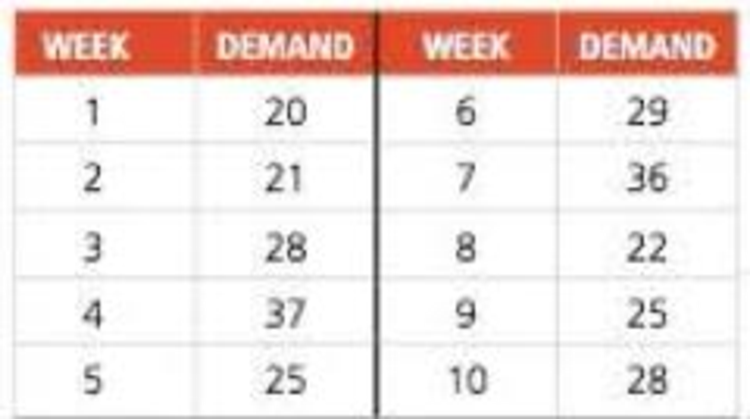
Sales of tablet computers at Ted Glickman’s electronics store in Washington, D.C., over the past 10 weeks are shown in the table below:
a)
b) Compute the MAD.
c) Compute the tracking signal.
a)
To determine: To forecast the demand for 10 weeks using exponential smoothing.
Introduction: A sequence of data points in successive order is known as time series. Time series forecasting is the prediction based on past events, which are at a uniform time interval. Exponential smoothing is one of the time series methods which use a smoothing constant to emphasis past data.
Answer to Problem 59P
Using exponential smoothing, the forecast for week 10 is done.
Explanation of Solution
Given information:
| Week | Demand |
| 1 | 20 |
| 2 | 21 |
| 3 | 28 |
| 4 | 37 |
| 5 | 25 |
| 6 | 29 |
| 7 | 36 |
| 8 | 22 |
| 9 | 25 |
| 10 | 28 |
Formula to calculate the forecasted demand:
Where,
Calculation to forecast demand using exponential smoothing:
| Week | Demand | Ft |
| 1 | 20 | 20 |
| 2 | 21 | 20 |
| 3 | 28 | 20.50 |
| 4 | 37 | 24.25 |
| 5 | 25 | 30.63 |
| 6 | 29 | 27.81 |
| 7 | 36 | 28.41 |
| 8 | 22 | 32.20 |
| 9 | 25 | 27.10 |
| 10 | 28 | 26.05 |
Excel worksheet:
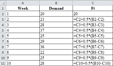
Calculation of the forecast for week 2:
To calculate the forecast for week 2, substitute the value of forecast of week 1, smoothing constant and difference between actual and forecasted demand in the above formula. The result of forecast for week 2 is 20.
Calculation of the forecast for week 3:
To calculate the forecast for week 3, substitute the value of forecast of week 1, smoothing constant and difference between actual and forecasted demand in the above formula. The result of forecast for week 3 is 20.50.
Calculation of the forecast for week 4:
To calculate the forecast for week 4, substitute the value of forecast of week 3, smoothing constant and difference between actual and forecasted demand in the above formula. The result of forecast for week 4 is 24.25.
Calculation of the forecast for week 5:
To calculate the forecast for week 5, substitute the value of forecast of week 4, smoothing constant and difference between actual and forecasted demand in the above formula. The result of forecast for week 5 is 30.63.
Calculation of the forecast for week 6:
To calculate the forecast for week 6, substitute the value of forecast of week 5, smoothing constant and difference between actual and forecasted demand in the above formula. The result of forecast for week 6 is 27.81.
Calculation of the forecast for week 7:
To calculate the forecast for week 7, substitute the value of forecast of week 6, smoothing constant and difference between actual and forecasted demand in the above formula. The result of forecast for week 7 is 28.41.
Calculation of the forecast for week 8:
To calculate the forecast for week 8, substitute the value of forecast of week 7, smoothing constant and difference between actual and forecasted demand in the above formula. The result of forecast for week 8 is 32.20.
Calculation of the forecast for week 9:
To calculate the forecast for week 9, substitute the value of forecast of year 8, smoothing constant and difference between actual and forecasted demand in the above formula. The result of forecast for week 9 is 27.10.
Calculation of the forecast for week 10:
To calculate the forecast for week 10, substitute the value of forecast of year 9, smoothing constant and difference between actual and forecasted demand in the above formula. The result of forecast for week 10 is 26.05.
Thus, using exponential smoothing, the forecast for week 10 is done.
b)
To determine: To compute MAD.
Answer to Problem 59P
MAD is 4.99.
Explanation of Solution
Given information:
| Week | Demand |
| 1 | 20 |
| 2 | 21 |
| 3 | 28 |
| 4 | 37 |
| 5 | 25 |
| 6 | 29 |
| 7 | 36 |
| 8 | 22 |
| 9 | 25 |
| 10 | 28 |
Formula to calculate MAD:
Calculation of MAD:
| Week | Demand | Ft | Absolute error |
| 1 | 20 | 20 | 0 |
| 2 | 21 | 20 | 1 |
| 3 | 28 | 20.50 | 7.50 |
| 4 | 37 | 24.25 | 12.75 |
| 5 | 25 | 30.63 | 5.63 |
| 6 | 29 | 27.81 | 1.19 |
| 7 | 36 | 28.41 | 7.59 |
| 8 | 22 | 32.20 | 10.20 |
| 9 | 25 | 27.10 | 2.10 |
| 10 | 28 | 26.05 | 1.95 |
| Total | 49.91 | ||
| MAD | 4.99 | ||
Table 1
Excel worksheet:
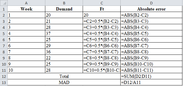
Calculation of the absolute error for week 2:
The absolute error for week 1 is the modulus of the difference between 21 and 20, which corresponds to 1. Therefore, the absolute error for week 2 is 1.
Calculation of the absolute error for week 3:
The absolute error for week 3 is the modulus of the difference between 28 and 20.50, which corresponds to 7.50. Therefore, the absolute error for week 3 is 7.50.
Calculation of the absolute error for week 4:
The absolute error for week 4 is the modulus of the difference between 37 and 24.25, which corresponds to 12.75. Therefore, the absolute error for week 4 is 12.75.
Calculation of the absolute error for week 5:
The absolute error for week 5 is the modulus of the difference between 25 and 30.63, which corresponds to 5.63. Therefore, the absolute error for week 5 is 5.63.
Calculation of the absolute error for week 6:
The absolute error for week 6 is the modulus of the difference between 29 and 27.81, which corresponds to 1.19. Therefore, the absolute error for week 6 is 1.19.
Calculation of the absolute error for week 7:
The absolute error for week 7 is the modulus of the difference between 36 and 28.41, which corresponds to 7.59. Therefore, the absolute error for week 7 is 7.59.
Calculation of the absolute error for week 8:
The absolute error for week 8 is the modulus of the difference between 22 and 32.20, which corresponds to 10.20. Therefore, the absolute error for week 8 is 10.20.
Calculation of the absolute error for week 9:
The absolute error for week 9 is the modulus of the difference between 25 and 27.10, which corresponds to 2.10. Therefore, the absolute error for week 9 is 2.10.
Calculation of the absolute error for week 10:
The absolute error for week 10 is the modulus of the difference between 28 and 26.05, which corresponds to 2.10. Therefore, the absolute error for week 10 is 2.10.
Calculation of the Mean Absolute Deviation:
The substitution of the summation value of absolute error for 10 weeks, divided by the number of weeks, which is 10 yields a MAD of 4.99.
The computed MAD is 4.99.
c)
To determine: To compute the tracking signal.
Answer to Problem 59P
The tracking signal is 2.82.
Explanation of Solution
Given information:
| Week | Demand |
| 1 | 20 |
| 2 | 21 |
| 3 | 28 |
| 4 | 37 |
| 5 | 25 |
| 6 | 29 |
| 7 | 36 |
| 8 | 22 |
| 9 | 25 |
| 10 | 28 |
Formula to calculate tracking signal:
Calculation of tracking signal:
Table 1 shows the calculation of MAD
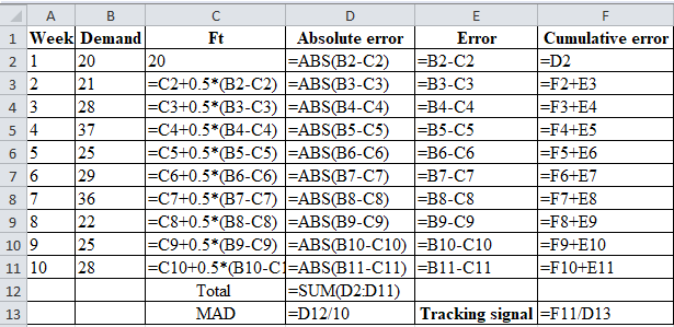
| Week | Demand | Ft | Absolute error | Error | Cumulative error |
| 1 | 20 | 20 | 0 | 0 | 0 |
| 2 | 21 | 20 | 1 | 1 | 1 |
| 3 | 28 | 20.50 | 7.50 | 7.5 | 8.50 |
| 4 | 37 | 24.25 | 12.75 | 12.75 | 21.25 |
| 5 | 25 | 30.63 | 5.63 | -5.63 | 15.63 |
| 6 | 29 | 27.81 | 1.19 | 1.19 | 16.81 |
| 7 | 36 | 28.41 | 7.59 | 7.59 | 24.41 |
| 8 | 22 | 32.20 | 10.20 | -10.20 | 14.20 |
| 9 | 25 | 27.10 | 2.10 | -2.10 | 12.10 |
| 10 | 28 | 26.05 | 1.95 | 1.95 | 14.05 |
| Total | 49.91 | ||||
| MAD | 4.99 | Tracking signal | 2.82 |
Excel worksheet:
Calculation of tracking signal:
The ratio of cumulative error and MAD is known as the tracking signal. The tracking signal of 2.82 is obtained by dividing 14.05 by 4.99.
Hence, the computed tracking signal is 2.82.
Want to see more full solutions like this?
Chapter 4 Solutions
EBK PRINCIPLES OF OPERATIONS MANAGEMENT


- Under what conditions might a firm use multiple forecasting methods?arrow_forwardScenario 4 Sharon Gillespie, a new buyer at Visionex, Inc., was reviewing quotations for a tooling contract submitted by four suppliers. She was evaluating the quotes based on price, target quality levels, and delivery lead time promises. As she was working, her manager, Dave Cox, entered her office. He asked how everything was progressing and if she needed any help. She mentioned she was reviewing quotations from suppliers for a tooling contract. Dave asked who the interested suppliers were and if she had made a decision. Sharon indicated that one supplier, Apex, appeared to fit exactly the requirements Visionex had specified in the proposal. Dave told her to keep up the good work. Later that day Dave again visited Sharons office. He stated that he had done some research on the suppliers and felt that another supplier, Micron, appeared to have the best track record with Visionex. He pointed out that Sharons first choice was a new supplier to Visionex and there was some risk involved with that choice. Dave indicated that it would please him greatly if she selected Micron for the contract. The next day Sharon was having lunch with another buyer, Mark Smith. She mentioned the conversation with Dave and said she honestly felt that Apex was the best choice. When Mark asked Sharon who Dave preferred, she answered, Micron. At that point Mark rolled his eyes and shook his head. Sharon asked what the body language was all about. Mark replied, Look, I know youre new but you should know this. I heard last week that Daves brother-in-law is a new part owner of Micron. I was wondering how soon it would be before he started steering business to that company. He is not the straightest character. Sharon was shocked. After a few moments, she announced that her original choice was still the best selection. At that point Mark reminded Sharon that she was replacing a terminated buyer who did not go along with one of Daves previous preferred suppliers. Ethical decisions that affect a buyers ethical perspective usually involve the organizational environment, cultural environment, personal environment, and industry environment. Analyze this scenario using these four variables.arrow_forwardScenario 4 Sharon Gillespie, a new buyer at Visionex, Inc., was reviewing quotations for a tooling contract submitted by four suppliers. She was evaluating the quotes based on price, target quality levels, and delivery lead time promises. As she was working, her manager, Dave Cox, entered her office. He asked how everything was progressing and if she needed any help. She mentioned she was reviewing quotations from suppliers for a tooling contract. Dave asked who the interested suppliers were and if she had made a decision. Sharon indicated that one supplier, Apex, appeared to fit exactly the requirements Visionex had specified in the proposal. Dave told her to keep up the good work. Later that day Dave again visited Sharons office. He stated that he had done some research on the suppliers and felt that another supplier, Micron, appeared to have the best track record with Visionex. He pointed out that Sharons first choice was a new supplier to Visionex and there was some risk involved with that choice. Dave indicated that it would please him greatly if she selected Micron for the contract. The next day Sharon was having lunch with another buyer, Mark Smith. She mentioned the conversation with Dave and said she honestly felt that Apex was the best choice. When Mark asked Sharon who Dave preferred, she answered, Micron. At that point Mark rolled his eyes and shook his head. Sharon asked what the body language was all about. Mark replied, Look, I know youre new but you should know this. I heard last week that Daves brother-in-law is a new part owner of Micron. I was wondering how soon it would be before he started steering business to that company. He is not the straightest character. Sharon was shocked. After a few moments, she announced that her original choice was still the best selection. At that point Mark reminded Sharon that she was replacing a terminated buyer who did not go along with one of Daves previous preferred suppliers. What should Sharon do in this situation?arrow_forward
- Scenario 4 Sharon Gillespie, a new buyer at Visionex, Inc., was reviewing quotations for a tooling contract submitted by four suppliers. She was evaluating the quotes based on price, target quality levels, and delivery lead time promises. As she was working, her manager, Dave Cox, entered her office. He asked how everything was progressing and if she needed any help. She mentioned she was reviewing quotations from suppliers for a tooling contract. Dave asked who the interested suppliers were and if she had made a decision. Sharon indicated that one supplier, Apex, appeared to fit exactly the requirements Visionex had specified in the proposal. Dave told her to keep up the good work. Later that day Dave again visited Sharons office. He stated that he had done some research on the suppliers and felt that another supplier, Micron, appeared to have the best track record with Visionex. He pointed out that Sharons first choice was a new supplier to Visionex and there was some risk involved with that choice. Dave indicated that it would please him greatly if she selected Micron for the contract. The next day Sharon was having lunch with another buyer, Mark Smith. She mentioned the conversation with Dave and said she honestly felt that Apex was the best choice. When Mark asked Sharon who Dave preferred, she answered, Micron. At that point Mark rolled his eyes and shook his head. Sharon asked what the body language was all about. Mark replied, Look, I know youre new but you should know this. I heard last week that Daves brother-in-law is a new part owner of Micron. I was wondering how soon it would be before he started steering business to that company. He is not the straightest character. Sharon was shocked. After a few moments, she announced that her original choice was still the best selection. At that point Mark reminded Sharon that she was replacing a terminated buyer who did not go along with one of Daves previous preferred suppliers. What does the Institute of Supply Management code of ethics say about financial conflicts of interest?arrow_forwardScenario 3 Ben Gibson, the purchasing manager at Coastal Products, was reviewing purchasing expenditures for packaging materials with Jeff Joyner. Ben was particularly disturbed about the amount spent on corrugated boxes purchased from Southeastern Corrugated. Ben said, I dont like the salesman from that company. He comes around here acting like he owns the place. He loves to tell us about his fancy car, house, and vacations. It seems to me he must be making too much money off of us! Jeff responded that he heard Southeastern Corrugated was going to ask for a price increase to cover the rising costs of raw material paper stock. Jeff further stated that Southeastern would probably ask for more than what was justified simply from rising paper stock costs. After the meeting, Ben decided he had heard enough. After all, he prided himself on being a results-oriented manager. There was no way he was going to allow that salesman to keep taking advantage of Coastal Products. Ben called Jeff and told him it was time to rebid the corrugated contract before Southeastern came in with a price increase request. Who did Jeff know that might be interested in the business? Jeff replied he had several companies in mind to include in the bidding process. These companies would surely come in at a lower price, partly because they used lower-grade boxes that would probably work well enough in Coastal Products process. Jeff also explained that these suppliers were not serious contenders for the business. Their purpose was to create competition with the bids. Ben told Jeff to make sure that Southeastern was well aware that these new suppliers were bidding on the contract. He also said to make sure the suppliers knew that price was going to be the determining factor in this quote, because he considered corrugated boxes to be a standard industry item. Is Ben Gibson acting legally? Is he acting ethically? Why or why not?arrow_forwardScenario 3 Ben Gibson, the purchasing manager at Coastal Products, was reviewing purchasing expenditures for packaging materials with Jeff Joyner. Ben was particularly disturbed about the amount spent on corrugated boxes purchased from Southeastern Corrugated. Ben said, I dont like the salesman from that company. He comes around here acting like he owns the place. He loves to tell us about his fancy car, house, and vacations. It seems to me he must be making too much money off of us! Jeff responded that he heard Southeastern Corrugated was going to ask for a price increase to cover the rising costs of raw material paper stock. Jeff further stated that Southeastern would probably ask for more than what was justified simply from rising paper stock costs. After the meeting, Ben decided he had heard enough. After all, he prided himself on being a results-oriented manager. There was no way he was going to allow that salesman to keep taking advantage of Coastal Products. Ben called Jeff and told him it was time to rebid the corrugated contract before Southeastern came in with a price increase request. Who did Jeff know that might be interested in the business? Jeff replied he had several companies in mind to include in the bidding process. These companies would surely come in at a lower price, partly because they used lower-grade boxes that would probably work well enough in Coastal Products process. Jeff also explained that these suppliers were not serious contenders for the business. Their purpose was to create competition with the bids. Ben told Jeff to make sure that Southeastern was well aware that these new suppliers were bidding on the contract. He also said to make sure the suppliers knew that price was going to be the determining factor in this quote, because he considered corrugated boxes to be a standard industry item. As the Marketing Manager for Southeastern Corrugated, what would you do upon receiving the request for quotation from Coastal Products?arrow_forward
- Sales of tablet computers at Ted Glickman’s electron-ics store in Washington, D.C., over the past 10 weeks are shown in the table below: a) Forecast demand for each week, including week 10, usingexponential smoothing with a 5 .5 (initial forecast 5 20). b) Compute the MAD.c) Compute the tracking signal.arrow_forwardFollowing table shows the monthly sales of X-box consoles at a retail store in Kuwait: Answer the following questions based on the data given above. Show your calculations. a. What is the expected sales for the 8th month based on 3 period moving average? b. What is the expected sales for the 8th month based on exponential smoothing with α =0.2? c. Which of the above two forecasting method is better based on MSE?arrow_forward10. What is the approximate forecast for May using a four-month moving average? a.38 b.43 c.44 d. 47arrow_forward
- Use the sales data in the table ( attached Image) and apply the same forecast method when α = 0.1, 0.2, 0.3, 0.4, 0.5, 0.6, 0.7, 0.8, 0.9, and 1. What is the best value for α? What does the best value of α indicate or show in regards to the forecast model? (Hint: Use Microsoft Excel to solve the question)arrow_forward12. Under the bottom-up approach, a central person or persons take the responsibility for forecasting and preparing an overall forecast. Select one: True Falsearrow_forwardWeek CheeseburgerSales 1 354 2 344 3 368 4 317 5 361 Based on historical observations over the past five weeks, make a forecast for the next period using the following methods: simple average, three-period moving average, and exponential smoothing with α = 0.4, given a forecast of 326 cheeseburgers for the first week. (Round your answers to 2 decimal places,e.g. 250.25) Simple average: F6 = enter forecast using a simple average 3-Period moving average: F6 = enter forecast using 3-Period moving average Exponential smoothing: F6 = enter forecast using exponential smoothing If actual sales for week 6 turn out to be 365, compare the three forecasts using MAD. Which method performed best?(Calculate your answers using the error only in period 6.) MAD (simple average) = enter forecast using a simple average of MAD MAD (3-period moving average) = enter forecast using 3-period moving average of MAD MAD (exponential smoothing) = enter forecast using exponential…arrow_forward
 Contemporary MarketingMarketingISBN:9780357033777Author:Louis E. Boone, David L. KurtzPublisher:Cengage Learning
 MarketingMarketingISBN:9780357033791Author:Pride, William MPublisher:South Western Educational Publishing
 Purchasing and Supply Chain ManagementOperations ManagementISBN:9781285869681Author:Robert M. Monczka, Robert B. Handfield, Larry C. Giunipero, James L. PattersonPublisher:Cengage Learning