
Concept explainers
Videos
To determine: Find the forecast of sales using exponential smoothing with smoothing constant 0.6 and 0.9 and infer the effect of exponential smoothing on forecast. Using MAD, determine the accurate forecast of exponential smoothing with given smoothing constant 0.3, 0.6 and 0.9.
Introduction: A sequence of data points in successive order is known as time series. Time series
Answer to Problem 17P
On Comparing MAD from exponential smoothing with smoothing constant 0.3, 0.6 and 0.9 (refer to equations (1), (2) and (3)), it can be inferred that the MAD of exponential smoothing with smoothing constant is most accurate because of least value of MAD.
Explanation of Solution
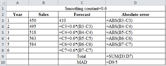
Forecast of sales using exponential smoothing with smoothing constant 0.6:
Given information:
| Year | Sales |
| 1 | 450 |
| 2 | 495 |
| 3 | 518 |
| 4 | 563 |
| 5 | 584 |
Formula to calculate the forecasted demand:
Where,
| Smoothing constant=0.6 | |||
| Year | Sales | Forecast | Absolute error |
| 1 | 450 | 410 | 40 |
| 2 | 495 | 434 | 61 |
| 3 | 518 | 470.6 | 47.4 |
| 4 | 563 | 499.04 | 63.96 |
| 5 | 584 | 537.416 | 46.584 |
| 6 | 565.3664 | ||
| Total | 258.944 | ||
| MAD | 51.7888 | ||
Excel worksheet:
Calculation of the forecast for year 2:
To calculate the forecast for year 2, substitute the value of forecast of year 1, smoothing constant and the difference of actual and forecasted demand in the above formula. The result of the forecast for year 2 is 434.
Calculation of the forecast for year 3:
To calculate the forecast for year 3, substitute the value of forecast of year 2, smoothing constant and the difference of actual and forecasted demand in the above formula. The result of the forecast for year 3 is 470.6.
Calculation of the forecast for year 4:
To calculate the forecast for year 4, substitute the value of forecast of year 3, smoothing constant and the difference of actual and forecasted demand in the above formula. The result of the forecast for year 4 is 499.04.
Calculation of the forecast for year 5:
To calculate the forecast for year 5, substitute the value of forecast of year 4, smoothing constant and the difference of actual and forecasted demand in the above formula. The result of the forecast for year 5 is 537.416.
Calculation of the forecast for year 6:
To calculate the forecast for year 5, substitute the value of forecast of year 5, smoothing constant and the difference of actual and forecasted demand in the above formula. The result of the forecast for year 6 is 565.36.
Calculation of MAD using exponential smoothing with smoothing constant α=0.6:
Formula to calculate the Mean Absolute Deviation:
Calculation of the absolute error for year 1:
The absolute error for year 1 is the modulus of the difference between 450 and 410, which corresponds to 40. Therefore, the absolute error for year 1 is 40.
Calculation of the absolute error for year 2:
The absolute error for year 2 is the modulus of the difference between 495 and 434, which is correspond to 61. Therefore, the absolute error for year 2 is 61.
Calculation of the absolute error for year 3:
The absolute error for year 3 is the modulus of the difference between 518and 470.6, which is correspond to 47.4. Therefore, the absolute error for year 3 is 47.4.
Calculation of the absolute error for year 4:
The absolute error for year 4 is the modulus of the difference between 563and499.04, which is correspond to 63.96. Therefore, the absolute error for year 4 is 63.96.
Calculation of the absolute error for year 5:
The absolute error for year 5 is the modulus of the difference between 584and537.416, which is correspond to 46.584. Therefore, the absolute error for year 5 is 46.584.
Calculation of the Mean Absolute Deviation using exponential smoothing with smoothing constant 0.6:
Upon the substitution of summation value of the absolute error for 5 years, that is, 258.944 is divided by the number of years. That is, 5 yields MAD of 51.7888.
The forecast of sales using exponential smoothing with 0.6 as smoothing constant is 565.36 and MAD is 51.7888.
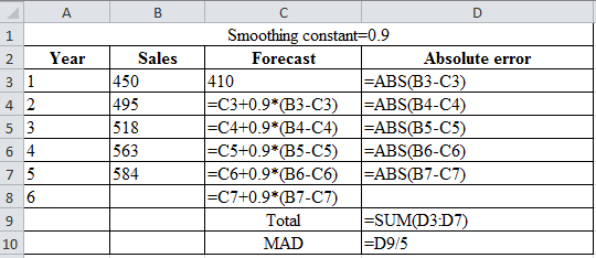
Forecast of sales using exponential smoothing with smoothing constant 0.9:
Given information:
| Year | Sales |
| 1 | 450 |
| 2 | 495 |
| 3 | 518 |
| 4 | 563 |
| 5 | 584 |
Formula to calculate the forecasted demand:
Where,
| Smoothing constant=0.9 | |||
| Year | Sales | Forecast | Absolute error |
| 1 | 450 | 410 | 40 |
| 2 | 495 | 446 | 49 |
| 3 | 518 | 490.1 | 27.9 |
| 4 | 563 | 515.21 | 47.79 |
| 5 | 584 | 558.221 | 25.779 |
| 6 | 581.4221 | ||
| Total | 190.469 | ||
| MAD | 38.0938 | ||
Excel worksheet:
Calculation of the forecast for year 2:
To calculate the forecast for year 2, substitute the value of forecast of year 1, smoothing constant and difference of actual and forecasted demand in the above formula. The result of the forecast for year 2 is 446.
Calculation of the forecast for year 3:
To calculate the forecast for year 3, substitute the value of forecast of year 2, smoothing constant and difference of actual and forecasted demand in the above formula. The result of the forecast for year 3 is 490.1.
Calculation of the forecast for year 4:
To calculate the forecast for year 4, substitute the value of forecast of year 3, smoothing constant and difference of actual and forecasted demand in the above formula. The result of the forecast for year 4 is 515.21.
Calculation of the forecast for year 5:
To calculate the forecast for year 5, substitute the value of forecast of year 4, smoothing constant and difference of actual and forecasted demand in the above formula. The result of forecast for year 5 is 558.221.
Calculation of the forecast for year 6:
To calculate the forecast for year 6, substitute the value of forecast of year 5, smoothing constant and difference of actual and forecasted demand in the above formula. The result of forecast for year 6 is 581.42.
Calculation of MAD using exponential smoothing with smoothing constant α=0.9:
Formula to calculate the Mean Absolute Deviation:
Calculation of the absolute error for year 1:
The absolute error for year 1 is the modulus of the difference between 450 and 410, which corresponds to 40. Therefore, the absolute error for year 1 is 40.
Calculation of the absolute error for year 2:
The absolute error for year 2 is the modulus of the difference between 495 and 446, which corresponds to 49. Therefore, the absolute error for year 2 is 49.
Calculation of the absolute error for year 3:
The absolute error for year 3 is the modulus of the difference between 518and490.1, which corresponds to 27.9. Therefore, the absolute error for year 3 is 27.9.
Calculation of the absolute error for year 4:
The absolute error for year 4 is the modulus of the difference between 563and515.21, which corresponds to 4.254. Therefore, the absolute error for year 4 is 47.79.
Calculation of the absolute error for year 5:
The absolute error for year 5 is the modulus of the difference between 584and558.221, which corresponds to 25.779. Therefore, the absolute error for year 5 is 25.779.
Calculation of the Mean Absolute Deviation using exponential smoothing:
Upon the substitution of summation value of absolute error for 5 years, that is, 190.469 is divided by the number of years. That is, 5 yields MAD of 38.093.
The forecast of sales using exponential smoothing with 0.9 as smoothing constant is 581.4221 and MAD is 38.093.
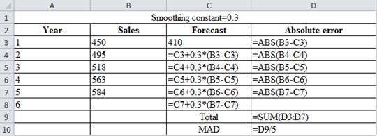
Forecast of sales using exponential smoothing with smoothing constant 0.3:
Given information:
| Year | Sales |
| 1 | 450 |
| 2 | 495 |
| 3 | 518 |
| 4 | 563 |
| 5 | 584 |
Formula to calculate the forecasted demand:
Where,
| Smoothing constant=0.3 | |||
| Year | Sales | Forecast | Absolute error |
| 1 | 450 | 410 | 40 |
| 2 | 495 | 422 | 73 |
| 3 | 518 | 443.9 | 74.1 |
| 4 | 563 | 466.13 | 96.87 |
| 5 | 584 | 495.191 | 88.809 |
| 6 | 521.8337 | ||
| Total | 372.779 | ||
| MAD | 74.5558 | ||
Excel worksheet:
Calculation of the forecast for year 2:
To calculate the forecast for year 2, substitute the value of forecast of year 1, smoothing constant and difference of actual and forecasted demand in the above formula. The result of the forecast for year 2 is 422.
Calculation of the forecast for year 3:
To calculate the forecast for year 3, substitute the value of forecast of year 2, smoothing constant and difference of actual and forecasted demand in the above formula. The result of the forecast for year 3 is 443.9.
Calculation of the forecast for year 4:
To calculate the forecast for year 4, substitute the value of forecast of year 3, smoothing constant and difference of actual and forecasted demand in the above formula. The result of the forecast for year 4 is 466.13.
Calculation of the forecast for year 5:
To calculate the forecast for year 5, substitute the value of forecast of year 4, smoothing constant and difference of actual and forecasted demand in the above formula. The result of the forecast for year 5 is 495.191.
Calculation of the forecast for year 6:
To calculate the forecast for year 6, substitute the value of forecast of year 5, smoothing constant and difference of actual and forecasted demand in the above formula. The result of the forecast for year 6 is 521.833.
Calculation of MAD using exponential smoothing with smoothing constant α=0.3:
Formula to calculate the Mean Absolute Deviation:
Calculation of the absolute error for year 1:
The absolute error for year 1 is the modulus of the difference between 450 and 410, which corresponds to 40. Therefore, the absolute error for year 1 is 40.
Calculation of the absolute error for year 2:
The absolute error for year 2 is the modulus of the difference between 495 and 422, which corresponds to 73. Therefore, the absolute error for year 2 is 73.
Calculation of the absolute error for year 3:
The absolute error for year 3 is the modulus of the difference between 518 and 443.9, which corresponds to 74.1. Therefore, the absolute error for year 3 is 74.1.
Calculation of the absolute error for year 4:
The absolute error for year 4 is the modulus of the difference between 563 and 466.13, which corresponds to 96.87. Therefore, the absolute error for year 4 is 96.87.
Calculation of the absolute error for year 5:
The absolute error for year 5 is the modulus of the difference between 584 and 495.191, which corresponds to 88.809. Therefore, the absolute error for year 5 is 88.809.
Calculation of the Mean Absolute Deviation using exponential smoothing with 0.3 as smoothing constant:
Upon the substitution of summation value of absolute error for 5 years, that is, 372.779 are divided by the number of years. That is, 5 yields MAD of 74.5558.
The forecast of sales using exponential smoothing with 0.3 as smoothing constant is 521.833 and MAD is 74.5558.
Hence, on comparing MAD from exponential smoothing with smoothing constant 0.3, 0.6 and 0.9 (refer to equations (1), (2) and (3)), it can be inferred that MAD of exponential smoothing with smoothing constant is most accurate because of least MAD.
Want to see more full solutions like this?
Chapter 4 Solutions
EBK PRINCIPLES OF OPERATIONS MANAGEMENT


- Under what conditions might a firm use multiple forecasting methods?arrow_forwardThe file P13_42.xlsx contains monthly data on consumer revolving credit (in millions of dollars) through credit unions. a. Use these data to forecast consumer revolving credit through credit unions for the next 12 months. Do it in two ways. First, fit an exponential trend to the series. Second, use Holts method with optimized smoothing constants. b. Which of these two methods appears to provide the best forecasts? Answer by comparing their MAPE values.arrow_forwardThe Baker Company wants to develop a budget to predict how overhead costs vary with activity levels. Management is trying to decide whether direct labor hours (DLH) or units produced is the better measure of activity for the firm. Monthly data for the preceding 24 months appear in the file P13_40.xlsx. Use regression analysis to determine which measure, DLH or Units (or both), should be used for the budget. How would the regression equation be used to obtain the budget for the firms overhead costs?arrow_forward
- The owner of a restaurant in Bloomington, Indiana, has recorded sales data for the past 19 years. He has also recorded data on potentially relevant variables. The data are listed in the file P13_17.xlsx. a. Estimate a simple regression equation involving annual sales (the dependent variable) and the size of the population residing within 10 miles of the restaurant (the explanatory variable). Interpret R-square for this regression. b. Add another explanatory variableannual advertising expendituresto the regression equation in part a. Estimate and interpret this expanded equation. How does the R-square value for this multiple regression equation compare to that of the simple regression equation estimated in part a? Explain any difference between the two R-square values. How can you use the adjusted R-squares for a comparison of the two equations? c. Add one more explanatory variable to the multiple regression equation estimated in part b. In particular, estimate and interpret the coefficients of a multiple regression equation that includes the previous years advertising expenditure. How does the inclusion of this third explanatory variable affect the R-square, compared to the corresponding values for the equation of part b? Explain any changes in this value. What does the adjusted R-square for the new equation tell you?arrow_forwardThe file P13_29.xlsx contains monthly time series data for total U.S. retail sales of building materials (which includes retail sales of building materials, hardware and garden supply stores, and mobile home dealers). a. Is seasonality present in these data? If so, characterize the seasonality pattern. b. Use Winters method to forecast this series with smoothing constants = = 0.1 and = 0.3. Does the forecast series seem to track the seasonal pattern well? What are your forecasts for the next 12 months?arrow_forwardThe file P13_22.xlsx contains total monthly U.S. retail sales data. While holding out the final six months of observations for validation purposes, use the method of moving averages with a carefully chosen span to forecast U.S. retail sales in the next year. Comment on the performance of your model. What makes this time series more challenging to forecast?arrow_forward
- The file P13_26.xlsx contains the monthly number of airline tickets sold by the CareFree Travel Agency. a. Create a time series chart of the data. Based on what you see, which of the exponential smoothing models do you think will provide the best forecasting model? Why? b. Use simple exponential smoothing to forecast these data, using a smoothing constant of 0.1. c. Repeat part b, but search for the smoothing constant that makes RMSE as small as possible. Does it make much of an improvement over the model in part b?arrow_forwardThe file P13_28.xlsx contains monthly retail sales of U.S. liquor stores. a. Is seasonality present in these data? If so, characterize the seasonality pattern. b. Use Winters method to forecast this series with smoothing constants = = 0.1 and = 0.3. Does the forecast series seem to track the seasonal pattern well? What are your forecasts for the next 12 months?arrow_forwardThe file P13_02.xlsx contains five years of monthly data on sales (number of units sold) for a particular company. The company suspects that except for random noise, its sales are growing by a constant percentage each month and will continue to do so for at least the near future. a. Explain briefly whether the plot of the series visually supports the companys suspicion. b. By what percentage are sales increasing each month? c. What is the MAPE for the forecast model in part b? In words, what does it measure? Considering its magnitude, does the model seem to be doing a good job? d. In words, how does the model make forecasts for future months? Specifically, given the forecast value for the last month in the data set, what simple arithmetic could you use to obtain forecasts for the next few months?arrow_forward
- The number of fishing rods selling each day is given below. Perform analyses of the time series to determine which model should be used for forecasting. 3 day moving average analysis 4 day moving average analysis 3 day weighted moving average analysis with weights W1=0.2, W2=0.3 and W3=0.5 with W1 on the oldest data. Exponential smoothing analysis with A=0.3 Which model provides a better fit of the data? Forecast day 13 sales of fishing rods using the model chosen in part (e) Day Rods Sold 1 60 2 70 3 110 4 80 5 70 6 85 7 115 8 105 9 65 10 75 11 95 12 85 Please read the relevant article, found in the VLE, before answering the question. Discuss the process and findings of the study of the article. Suggest a possible study that could be done at your current or past job that could use a similar methodology and analysis.arrow_forwardCompute a 3-month weighted average forecast for months 4 through 9. Assign weights of 0.55, 0.33 and 0.12 to the months in sequence, starting with the most recent month. Compare the two forecasts using MAD. Which forecast is better the 3-month moving average or the 3-month weighted moving average and why?arrow_forwardBased on the following equation for a moving average forecast, what would have been the three week moving average forecast for week 53 for Small Town Restaurant (see downloaded file for actual demand)? Provide two decimal places and use normal rounding. What happens if we increase the time periods in our moving average forecast to six weeks opposed to three? Group of answer choices It would be more accurate because it includes more data. There would be no change. It would be less sensitive to changes. It would be better at predicting a trend.arrow_forward
 Practical Management ScienceOperations ManagementISBN:9781337406659Author:WINSTON, Wayne L.Publisher:Cengage,
 Contemporary MarketingMarketingISBN:9780357033777Author:Louis E. Boone, David L. KurtzPublisher:Cengage Learning
 MarketingMarketingISBN:9780357033791Author:Pride, William MPublisher:South Western Educational Publishing