
Videos
Bus and subway ridership for the summer months in London, England, is believed to be tied heavily to the number of tourists visiting the city. During the past 12 years, the data on the next page have been obtained:
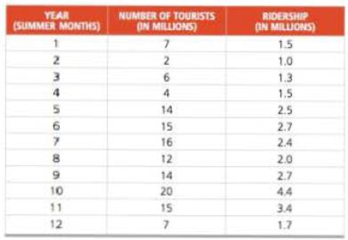
a) Plot these data and decide if a linear model is reasonable.
b) Develop a regression relationship.
c) What is expected ridership if 10 million tourists visit London in a year?
d) Explain the predicted ridership if there are no tourists at all.
e) What is the standard error of the estimate?
f) What is the model’s correlation coefficient and coefficient of determination?
a)
To determine: To plot the data and decide whether the linear model is reasonable.
Introduction: Forecasting is used to predict future changes or demand patterns. It involves different approaches and varies with different periods.
Answer to Problem 52P
The graph for the given data is plotted and it can be observed that the data points are scattered around.
Explanation of Solution
Given information:
| Year (Summer Months) | Number of tourist (in millions) | Ridership (in millions) |
| 1 | 7 | 1.5 |
| 2 | 2 | 1 |
| 3 | 6 | 1.3 |
| 4 | 4 | 1.5 |
| 5 | 14 | 2.5 |
| 6 | 15 | 2.7 |
| 7 | 16 | 2.4 |
| 8 | 12 | 2 |
| 9 | 14 | 2.7 |
| 10 | 20 | 4.4 |
| 11 | 15 | 3.4 |
| 12 | 7 | 1.7 |
Table 1
Graphical representation:
The data to plot the graph is taken from Table 1.
Hence, the graph for the given data is plotted and it can be observed that the data points are scattered around.
b)
To determine: A regression relationship.
Answer to Problem 52P
The linear regression equation is
Explanation of Solution
Given information:
| Year (Summer Months) | Number of tourist (in millions) | Ridership (in millions) |
| 1 | 7 | 1.5 |
| 2 | 2 | 1 |
| 3 | 6 | 1.3 |
| 4 | 4 | 1.5 |
| 5 | 14 | 2.5 |
| 6 | 15 | 2.7 |
| 7 | 16 | 2.4 |
| 8 | 12 | 2 |
| 9 | 14 | 2.7 |
| 10 | 20 | 4.4 |
| 11 | 15 | 3.4 |
| 12 | 7 | 1.7 |
Formula of least square regression:
Where,
Where,
| Year (Summer Months) | Number of tourist (in millions) (x) | Ridership (in millions) (y) | xy | x^2 | y^2 |
| 1 | 7 | 1.5 | 10.5 | 49 | 2.25 |
| 2 | 2 | 1 | 2 | 4 | 1 |
| 3 | 6 | 1.3 | 7.8 | 36 | 1.69 |
| 4 | 4 | 1.5 | 6 | 16 | 2.25 |
| 5 | 14 | 2.5 | 35 | 196 | 6.25 |
| 6 | 15 | 2.7 | 40.5 | 225 | 7.29 |
| 7 | 16 | 2.4 | 38.4 | 256 | 5.76 |
| 8 | 12 | 2 | 24 | 144 | 4 |
| 9 | 14 | 2.7 | 37.8 | 196 | 7.29 |
| 10 | 20 | 4.4 | 88 | 400 | 19.36 |
| 11 | 15 | 3.4 | 51 | 225 | 11.56 |
| 12 | 7 | 1.7 | 11.9 | 49 | 2.89 |
| Total | 132 | 27.1 | 352.9 | 1796 | 71.59 |
Table 2
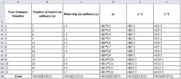
Excel worksheet:
Substitute the values in the above formula.
Calculation of the average of x values
The average of x values is obtained by dividing the summation of x values with the number of periods n=12, the value of
Calculation of the average of y values
The average of y values is obtained by dividing the summation of sales with the number of periods n=12. The value of
Calculation ofthe slope of regression line‘b’:
The summation of the product of sales (y) with x values is ∑xy = 352.9, the product of number of period (n), the average of x values and the average of y values is obtained;
The summation of the square of x values, 1796, is subtracted from the product of the number of periods, 10with the average of x values, 11. The resultant value is 344. The slope of the regression line is obtained by dividing 1796 with 344. The value of ‘b’ is 0.159.
Calculation of the y-axis intercept ‘a’:
The y-axis intercept is obtained by the difference between the average of y values and values obtained by the product of the slope of regression line with the average of x values. The resultant value of ‘a’ is 0.511.
Least Square Regression forecasting equation:
Substitute the slope of regression line and they axis intercept in the regression equation which gives the liner regression equation for the data.
Hence, the linear regression equation is
c)
To determine: The expected ridership when 10 million tourists visit in a year.
Answer to Problem 52P
There is a 2.101 million ridership when 10 million tourists visit in a year.
Explanation of Solution
Given information:
| Year (Summer Months) | Number of tourist (in millions) | Ridership (in millions) |
| 1 | 7 | 1.5 |
| 2 | 2 | 1 |
| 3 | 6 | 1.3 |
| 4 | 4 | 1.5 |
| 5 | 14 | 2.5 |
| 6 | 15 | 2.7 |
| 7 | 16 | 2.4 |
| 8 | 12 | 2 |
| 9 | 14 | 2.7 |
| 10 | 20 | 4.4 |
| 11 | 15 | 3.4 |
| 12 | 7 | 1.7 |
Formula of least square regression:
Where,
Where,
Calculation of number of ridership when 10 million touristsvisit in a year:
Equation (1) provides the linear regression equation for the data and substitutes the number of tourists visiting in the regression equation. Substituting 10 million in the equation, the resultant value is found to be 2.101 million ridership.
Hence, there are 2.101 million ridership when 10 million touristsvisit in a year.
d)
To determine: The expected ridership when no tourists visit in a year.
Answer to Problem 52P
There is a 511,000 ridership when no touristsvisit in a year.
Explanation of Solution
Given information:
| Year (Summer Months) | Number of tourist (in millions) | Ridership (in millions) |
| 1 | 7 | 1.5 |
| 2 | 2 | 1 |
| 3 | 6 | 1.3 |
| 4 | 4 | 1.5 |
| 5 | 14 | 2.5 |
| 6 | 15 | 2.7 |
| 7 | 16 | 2.4 |
| 8 | 12 | 2 |
| 9 | 14 | 2.7 |
| 10 | 20 | 4.4 |
| 11 | 15 | 3.4 |
| 12 | 7 | 1.7 |
Formula of least square regression:
Where,
Where,
Calculation of the number of ridership when notouristsvisit in a year:
Equation (1) provides the linear regression equation for the data and substitutes the number of tourists visiting in the regression equation. Substituting 0 in the equation, the resultant value is 0.511 million ridership.
Hence, there is a 511,000 ridership when notouristsvisit in a year.
e)
To determine: The standard error of estimate.
Answer to Problem 52P
The standard error of estimate is0.4037.
Explanation of Solution
Given information:
| Year (Summer Months) | Number of tourists(in millions) | Ridership (in millions) |
| 1 | 7 | 1.5 |
| 2 | 2 | 1 |
| 3 | 6 | 1.3 |
| 4 | 4 | 1.5 |
| 5 | 14 | 2.5 |
| 6 | 15 | 2.7 |
| 7 | 16 | 2.4 |
| 8 | 12 | 2 |
| 9 | 14 | 2.7 |
| 10 | 20 | 4.4 |
| 11 | 15 | 3.4 |
| 12 | 7 | 1.7 |
Formula to compute the standard error of estimate:
Calculation of standard error of estimate:
The values to be substituted in the standard error of estimate formula are given inTable 2. Substitute the values from the table in the formula. This results in a standard error of estimate of 0.4037.
Hence, the standard error of estimate is 0.4037.
f)
To determine: The coefficient of correlation (r) and coefficient of determination (r2).
Answer to Problem 52P
The coefficient of correlation (r) and coefficient of determination (r2) are 717.41 & 0.840, respectively.
Explanation of Solution
Given information:
| Year (Summer Months) | Number of tourists(in millions) | Ridership (in millions) |
| 1 | 7 | 1.5 |
| 2 | 2 | 1 |
| 3 | 6 | 1.3 |
| 4 | 4 | 1.5 |
| 5 | 14 | 2.5 |
| 6 | 15 | 2.7 |
| 7 | 16 | 2.4 |
| 8 | 12 | 2 |
| 9 | 14 | 2.7 |
| 10 | 20 | 4.4 |
| 11 | 15 | 3.4 |
| 12 | 7 | 1.7 |
Formula to calculate the correlation coefficient:
Calculation of the correlation coefficient (r):
Table (2) provides the values to calculate the correlation coefficient (r).
Calculation of the correlation of determination (r2):
Hence, the coefficient of correlation and coefficient of determination are 717.41 and 0.840, respectively.
Want to see more full solutions like this?
Chapter 4 Solutions
EBK PRINCIPLES OF OPERATIONS MANAGEMENT


- The owner of a restaurant in Bloomington, Indiana, has recorded sales data for the past 19 years. He has also recorded data on potentially relevant variables. The data are listed in the file P13_17.xlsx. a. Estimate a simple regression equation involving annual sales (the dependent variable) and the size of the population residing within 10 miles of the restaurant (the explanatory variable). Interpret R-square for this regression. b. Add another explanatory variableannual advertising expendituresto the regression equation in part a. Estimate and interpret this expanded equation. How does the R-square value for this multiple regression equation compare to that of the simple regression equation estimated in part a? Explain any difference between the two R-square values. How can you use the adjusted R-squares for a comparison of the two equations? c. Add one more explanatory variable to the multiple regression equation estimated in part b. In particular, estimate and interpret the coefficients of a multiple regression equation that includes the previous years advertising expenditure. How does the inclusion of this third explanatory variable affect the R-square, compared to the corresponding values for the equation of part b? Explain any changes in this value. What does the adjusted R-square for the new equation tell you?arrow_forwardThe Baker Company wants to develop a budget to predict how overhead costs vary with activity levels. Management is trying to decide whether direct labor hours (DLH) or units produced is the better measure of activity for the firm. Monthly data for the preceding 24 months appear in the file P13_40.xlsx. Use regression analysis to determine which measure, DLH or Units (or both), should be used for the budget. How would the regression equation be used to obtain the budget for the firms overhead costs?arrow_forwardUnder what conditions might a firm use multiple forecasting methods?arrow_forward
- A small computer chip manufacturer wants to forecast monthly ozperating costs as a function of the number of units produced during a month. The company has collected the 16 months of data in the file P13_34.xlsx. a. Determine an equation that can be used to predict monthly production costs from units produced. Are there any outliers? b. How could the regression line obtained in part a be used to determine whether the company was efficient or inefficient during any particular month?arrow_forwardDo the sales prices of houses in a given community vary systematically with their sizes (as measured in square feet)? Answer this question by estimating a simple regression equation where the sales price of the house is the dependent variable, and the size of the house is the explanatory variable. Use the sample data given in P13_06.xlsx. Interpret your estimated equation, the associated R-square value, and the associated standard error of estimate.arrow_forwardStock market analysts are continually looking for reliable predictors of stock prices. Consider the problem of modeling the price per share of electric utility stocks (Y). Two variables thought to influence this stock price are return on average equity (X1) and annual dividend rate (X2). The stock price, returns on equity, and dividend rates on a randomly selected day for 16 electric utility stocks are provided in the file P13_15.xlsx. Estimate a multiple regression equation using the given data. Interpret each of the estimated regression coefficients. Also, interpret the standard error of estimate and the R-square value for these data.arrow_forward
- Suppose that a regional express delivery service company wants to estimate the cost of shipping a package (Y) as a function of cargo type, where cargo type includes the following possibilities: fragile, semifragile, and durable. Costs for 15 randomly chosen packages of approximately the same weight and same distance shipped, but of different cargo types, are provided in the file P13_16.xlsx. a. Estimate a regression equation using the given sample data, and interpret the estimated regression coefficients. b. According to the estimated regression equation, which cargo type is the most costly to ship? Which cargo type is the least costly to ship? c. How well does the estimated equation fit the given sample data? How might the fit be improved? d. Given the estimated regression equation, predict the cost of shipping a package with semifragile cargo.arrow_forwardThe file P13_42.xlsx contains monthly data on consumer revolving credit (in millions of dollars) through credit unions. a. Use these data to forecast consumer revolving credit through credit unions for the next 12 months. Do it in two ways. First, fit an exponential trend to the series. Second, use Holts method with optimized smoothing constants. b. Which of these two methods appears to provide the best forecasts? Answer by comparing their MAPE values.arrow_forwardThe management of a technology company is trying to determine the variable that best explains the variation of employee salaries using a sample of 52 full-time employees; see the file P13_08.xlsx. Estimate simple linear regression equations to identify which of the following has the strongest linear relationship with annual salary: the employees gender, age, number of years of relevant work experience prior to employment at the company, number of years of employment at the company, or number of years of post secondary education. Provide support for your conclusion.arrow_forward
- Mark Gershon, owner of a musical instrument distributorship, thinks that demand for guitars may be related to the number of television appearances by the popular group Maroon 5 during the previous month. Gershon has collected the data shown in the following table: Maroon 5 Tv Appearances 3 4 7 6 8 5 Demand for Guitars 3 6 7 5 10 7 b) Using the least-squares regression method, the equation for forecasting is (round your response to four decimal places): Y= _____+_____X C) The estimate for guitar sales if Maroon 5 performed on Tv 9 times =___ (round your response to 2 decimal placesarrow_forwardThe manager of the Salem police department motor poolwants to develop a forecast model for annual maintenanceon police cars based on mileage in the past year and age ofthe cars. The following data have been collected for eightdifferent cars: a. Using Excel develop a multiple regression equationfor these data.b. What is the coefficient of determination for thisregression equation?c. Forecast the annual maintenance cost for a police carthat is four years old and will be driven 10,000 miles inone year.arrow_forwardCalculate a regression line for the data and indicate the forecast of sales for a store with advertising spending of R240,000? and R300,000? Store Advertising Sales 1 14 6 2 11 3 3 15 5 4 16 5 5 24 15 6 28 18 7 22 17 8 21 12 9 26 15 10 43 20 11 34 14 12 9 5arrow_forward
 Practical Management ScienceOperations ManagementISBN:9781337406659Author:WINSTON, Wayne L.Publisher:Cengage,
 Contemporary MarketingMarketingISBN:9780357033777Author:Louis E. Boone, David L. KurtzPublisher:Cengage Learning
 MarketingMarketingISBN:9780357033791Author:Pride, William MPublisher:South Western Educational Publishing