
Concept explainers
Videos
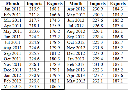
Imports and exports: The following table presents the U.S. imports and exports (in billions of dollars) for each of 29 months.
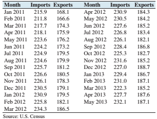
- Compute the least-squares regression line for predicting exports (y) from imports (x).
- Compute the coefficient of determination.
- The months with the two lowest exports are January and February 2011 Remove these points and compute the least-squares regression line. Is the result noticeably different?
- Compute the coefficient of determination for the data set with January and February 2011 removed.
- Two economists decide to study the relationship between imports and exports. One uses data from January 2011 through May 2013 and the other used data from March 2011 through May 2013. For which data set will the proportion of variance explained by the least-squares regression line be greater?
(a)
>The least squares regression line for the given data set.
Answer to Problem 26E
Explanation of Solution
Given information:
The following table presents the U.S. imports and exports (in billions of dollars) for each of
months:
Concepts Used:
The equation for least-square regression line:
Where
The correlation coefficient of a data is given by:
Where,
The standard deviations are given by:
Calculation:
The mean of
The mean of
The data can be represented in tabular form as:
| x | y |  |
 |
 |
 |
 |
| 215.9 | 168.1 | -10.21724 | 104.39202 | -13.18276 | 173.78512 | 134.69143 |
| 211.8 | 166.6 | -14.31724 | 204.98340 | -14.68276 | 215.58340 | 210.21660 |
| 217.7 | 174.3 | -8.41724 | 70.84995 | -6.98276 | 48.75892 | 58.77556 |
| 218.1 | 175.9 | -8.01724 | 64.27616 | -5.38276 | 28.97409 | 43.15488 |
| 223.6 | 176.2 | -2.51724 | 6.33650 | -5.08276 | 25.83444 | 12.79453 |
| 224.2 | 173.2 | -1.91724 | 3.67581 | -8.08276 | 65.33099 | 15.49660 |
| 224.9 | 179.5 | -1.21724 | 1.48168 | -1.78276 | 3.17823 | 2.17005 |
| 224.6 | 179.9 | -1.51724 | 2.30202 | -1.38276 | 1.91202 | 2.09798 |
| 225.7 | 181.2 | -0.41724 | 0.17409 | -0.08276 | 0.00685 | 0.03453 |
| 226.6 | 180.5 | 0.48276 | 0.23306 | -0.78276 | 0.61271 | -0.37788 |
| 226.1 | 178.3 | -0.01724 | 0.00030 | -2.98276 | 8.89685 | 0.05143 |
| 230.5 | 179.1 | 4.38276 | 19.20857 | -2.18276 | 4.76444 | -9.56650 |
| 230.9 | 179.5 | 4.78276 | 22.87478 | -1.78276 | 3.17823 | -8.52650 |
| 225.8 | 182.1 | -0.31724 | 0.10064 | 0.81724 | 0.66788 | -0.25926 |
| 234.3 | 186.5 | 8.18276 | 66.95754 | 5.21724 | 27.21961 | 42.69143 |
| 230.9 | 184.3 | 4.78276 | 22.87478 | 3.01724 | 9.10375 | 14.43074 |
| 230.5 | 184.2 | 4.38276 | 19.20857 | 2.91724 | 8.51030 | 12.78556 |
| 227.6 | 185.2 | 1.48276 | 2.19857 | 3.91724 | 15.34478 | 5.80832 |
| 226.8 | 183.4 | 0.68276 | 0.46616 | 2.11724 | 4.48271 | 1.44556 |
| 226.1 | 182.1 | -0.01724 | 0.00030 | 0.81724 | 0.66788 | -0.01409 |
| 228.4 | 186.8 | 2.28276 | 5.21099 | 5.51724 | 30.43995 | 12.59453 |
| 225.3 | 182.7 | -0.81724 | 0.66788 | 1.41724 | 2.00857 | -1.15823 |
| 231.6 | 185.2 | 5.48276 | 30.06064 | 3.91724 | 15.34478 | 21.47729 |
| 227.0 | 188.7 | 0.88276 | 0.77926 | 7.41724 | 55.01547 | 6.54763 |
| 229.4 | 186.7 | 3.28276 | 10.77650 | 5.41724 | 29.34650 | 17.78350 |
| 231.0 | 187.1 | 4.88276 | 23.84133 | 5.81724 | 33.84030 | 28.40419 |
| 222.3 | 185.2 | -3.81724 | 14.57133 | 3.91724 | 15.34478 | -14.95306 |
| 227.7 | 187.6 | 1.58276 | 2.50512 | 6.31724 | 39.90754 | 9.99867 |
| 232.1 | 187.1 | 5.98276 | 35.79340 | 5.81724 | 33.84030 | 34.80315 |
|
|
|
|
|
|
Hence, the standard deviation is given by:
And,
Consider,
Putting the values in the formula,
Putting the values to obtain b1,
Putting the values to obtain b0,
Hence, the least-square regression line is given by:
Therefore, the least squares regression line for the given data set is
(b)
>The coefficient of determination.
Answer to Problem 26E
Explanation of Solution
Given information:
Same as part
Calculation:
From part
The coefficient of determination is given by:

Where
Putting the values to obtain Coefficient of Determination,
Therefore, the Coefficient of Determination is
(c)
>The least squares regression line for the given data set by excluding the outlier points and to check if the result is noticeably different.
Answer to Problem 26E
The result is noticeably different.
Explanation of Solution
Given information:
Same as part
The months with two lowest exports are January and February
Concepts used:
The equation for least-square regression line:
Where
The correlation coefficient of a data is given by:
Where,
The standard deviations are given by:
Calculation:
The months with two lowest exports are January and February
Excluding the outlier,
The mean of
The mean of
The data can be represented in tabular form as:
| x | y |  |
 |
 |
 |
 |
| 217.7 | 174.3 | -8.41724 | 70.84995 | -6.98276 | 48.75892 | 58.77556 |
| 218.1 | 175.9 | -8.01724 | 64.27616 | -5.38276 | 28.97409 | 43.15488 |
| 223.6 | 176.2 | -2.51724 | 6.33650 | -5.08276 | 25.83444 | 12.79453 |
| 224.2 | 173.2 | -1.91724 | 3.67581 | -8.08276 | 65.33099 | 15.49660 |
| 224.9 | 179.5 | -1.21724 | 1.48168 | -1.78276 | 3.17823 | 2.17005 |
| 224.6 | 179.9 | -1.51724 | 2.30202 | -1.38276 | 1.91202 | 2.09798 |
| 225.7 | 181.2 | -0.41724 | 0.17409 | -0.08276 | 0.00685 | 0.03453 |
| 226.6 | 180.5 | 0.48276 | 0.23306 | -0.78276 | 0.61271 | -0.37788 |
| 226.1 | 178.3 | -0.01724 | 0.00030 | -2.98276 | 8.89685 | 0.05143 |
| 230.5 | 179.1 | 4.38276 | 19.20857 | -2.18276 | 4.76444 | -9.56650 |
| 230.9 | 179.5 | 4.78276 | 22.87478 | -1.78276 | 3.17823 | -8.52650 |
| 225.8 | 182.1 | -0.31724 | 0.10064 | 0.81724 | 0.66788 | -0.25926 |
| 234.3 | 186.5 | 8.18276 | 66.95754 | 5.21724 | 27.21961 | 42.69143 |
| 230.9 | 184.3 | 4.78276 | 22.87478 | 3.01724 | 9.10375 | 14.43074 |
| 230.5 | 184.2 | 4.38276 | 19.20857 | 2.91724 | 8.51030 | 12.78556 |
| 227.6 | 185.2 | 1.48276 | 2.19857 | 3.91724 | 15.34478 | 5.80832 |
| 226.8 | 183.4 | 0.68276 | 0.46616 | 2.11724 | 4.48271 | 1.44556 |
| 226.1 | 182.1 | -0.01724 | 0.00030 | 0.81724 | 0.66788 | -0.01409 |
| 228.4 | 186.8 | 2.28276 | 5.21099 | 5.51724 | 30.43995 | 12.59453 |
| 225.3 | 182.7 | -0.81724 | 0.66788 | 1.41724 | 2.00857 | -1.15823 |
| 231.6 | 185.2 | 5.48276 | 30.06064 | 3.91724 | 15.34478 | 21.47729 |
| 227.0 | 188.7 | 0.88276 | 0.77926 | 7.41724 | 55.01547 | 6.54763 |
| 229.4 | 186.7 | 3.28276 | 10.77650 | 5.41724 | 29.34650 | 17.78350 |
| 231.0 | 187.1 | 4.88276 | 23.84133 | 5.81724 | 33.84030 | 28.40419 |
| 222.3 | 185.2 | -3.81724 | 14.57133 | 3.91724 | 15.34478 | -14.95306 |
| 227.7 | 187.6 | 1.58276 | 2.50512 | 6.31724 | 39.90754 | 9.99867 |
| 232.1 | 187.1 | 5.98276 | 35.79340 | 5.81724 | 33.84030 | 34.80315 |
|
|
|
|
|
|
Hence, the standard deviation is given by:
And,
Consider, 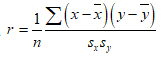
Putting the values in the formula,
Putting the values to obtain
Putting the values to obtain
Hence, the least-square regression line is given by:
Therefore, the least squares regression line for the given data set by removing the outlier is
Hence the result is noticeably different.
(d)
>The coefficient of determination for the data set with the outlier removed.
Answer to Problem 26E
Explanation of Solution
Given information:
Same as part
The months with two lowest exports are January and February
Calculation:
From part
The coefficient of determination is given by:
Where
Plugging the values to obtain Coefficient of Determination,
Therefore, the Coefficient of Determination is
(e)
>To calculate:
To check for which data set will the proportion of variance explained by the least-squares regression line be greater.
Answer to Problem 26E
The proportion of variance explained by the least-squares regression line is greater for the data from January
Explanation of Solution
Given information:
Same as part
Two economists decide to study the relationship between imports and exports. One uses data from January
Calculation:
From previous parts of this exercise,
The Coefficient of Determination is
The Coefficient of Determination without the outliers is
Here the coefficient of determination decreased without the outliers.
Hence, the proportion of variance explained is less without the outlier.
Therefore, the proportion of variance explained by the least-squares regression line is greater for the data from January
Want to see more full solutions like this?
Chapter 4 Solutions
ELEMENTARY STATISTICS LOOSE+ACCESS COD


 Elementary Linear Algebra (MindTap Course List)AlgebraISBN:9781305658004Author:Ron LarsonPublisher:Cengage Learning
 Linear Algebra: A Modern IntroductionAlgebraISBN:9781285463247Author:David PoolePublisher:Cengage Learning