
Videos
a.
Draw a
a.
Answer to Problem 18CRE
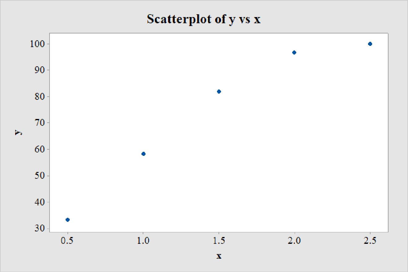
The scatterplot for the data is obtained as follows:
The relationship between the variables is nonlinear.
Explanation of Solution
Calculation:
The data on success (%), y and energy of shock, x is given.
Scatterplot:
Software procedure:
Step-by-step procedure to draw the scatterplot using MINITAB software is given below:
- Choose Graph > Scatterplot.
- Choose Simple, and then click OK.
- Enter the column of y under Y variables.
- Enter the column of x under X variables.
- Click OK.
Thus, the scatterplot is obtained.
A careful observation of the scatterplot reveals that for lower values of x, the points are close to being linear. However, the curvature in the distribution of the points gradually increases with increasing values of x.
Thus, the relationship between the variables is nonlinear.
b.
Fit a least-squares regression line to the data.
Construct a residual plot for the model.
Explain whether the residual plot supports the conclusion in Part a.
b.
Answer to Problem 18CRE
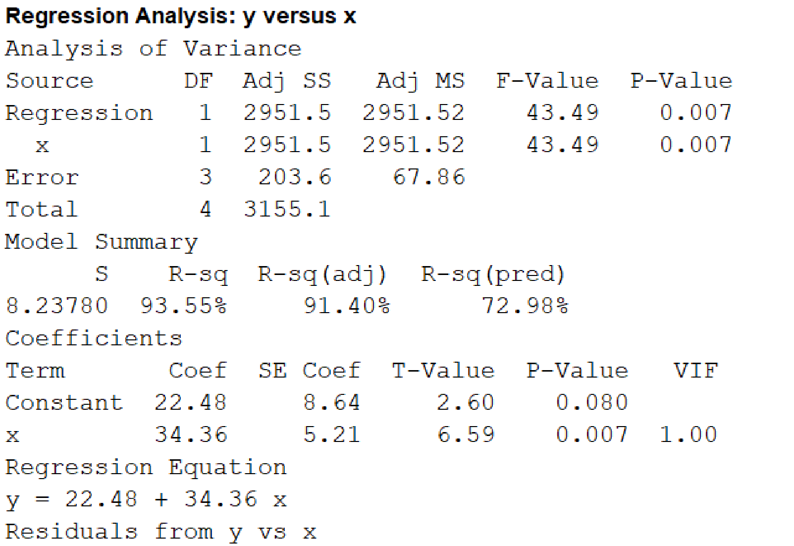
The least-squares regression line for the data is
Explanation of Solution
Calculation:
The least-squares regression line can be obtained using software.
Regression:
Software procedure:
Step by step procedure to get regression equation using MINITAB software is given as,
- Choose Stat > Regression > Regression > Fit Regression Model.
- Under Responses, enter the column of y.
- Under Continuous predictors, enter the columns of x.
- Choose Results and select Analysis of Variance, Model Summary, Coefficients, Regression Equation.
- Choose Graphs, under Residual versus the variables, enter x.
- Click OK on all dialogue boxes.
The outputs using MINITAB software is given as follows:
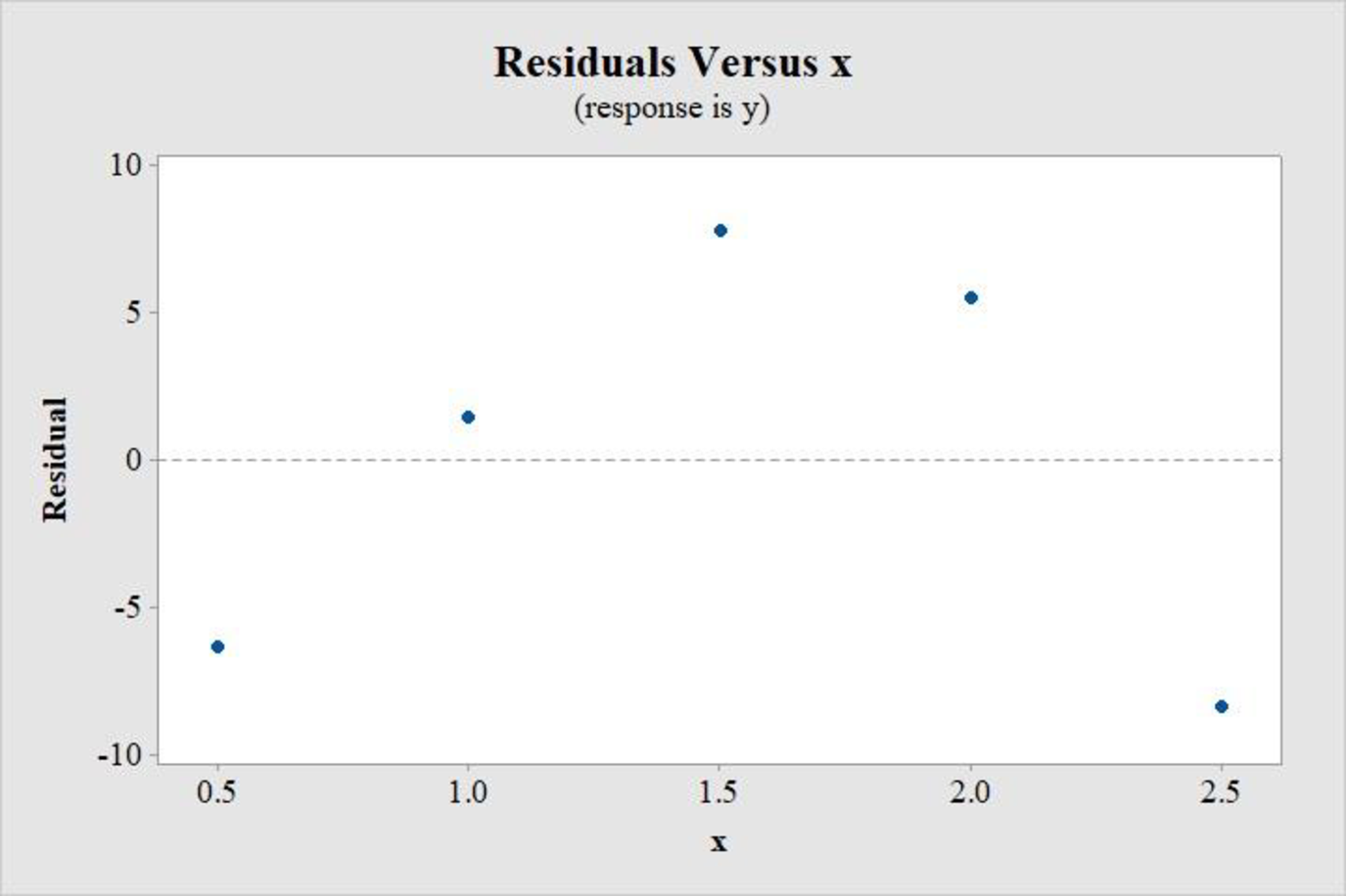
Residual plot:
From the output, the least-squares regression line is:
The ideal residual plot for a linear regression model must not show any pattern and must be randomly distributed. However, this residual plot clearly shows a curved pattern, with an approximate inverted U-shape. This suggests that the data is not linearly distributed.
Thus, the residual plot supports the conclusion in Part a.
c.
Justify whether the transformation
c.
Answer to Problem 18CRE
The transformation
Explanation of Solution
Calculation:
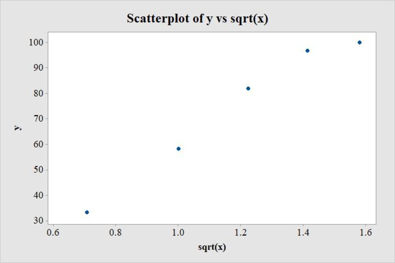
The suitable transformation can be identified by constructing scatterplot between y and
Consider the transformed variable,
Data transformation
Software procedure:
Step-by-step procedure to transform the data using MINITAB software is given below:
- Choose Calc > Calculator.
- Enter the column of sqrt(x) under Store result in variable.
- Enter the formula SQRT(‘x’) under Expression.
- Click OK.
The transformed variable is stored in the column sqrt(x).
Scatterplot:
Software procedure:
Step-by-step procedure to draw the scatterplot using MINITAB software is given below:
- Choose Graph > Scatterplot.
- Choose Simple, and then click OK.
- Enter the column of y under Y variables.
- Enter the column of sqrt(x) under X variables.
- Click OK.
The output obtained using MINITAB is as follows:
Consider the transformed variable,
Data transformation
Software procedure:
Step-by-step procedure to transform the data using MINITAB software is given below:
- Choose Calc > Calculator.
- Enter the column of sqrt(x) under Store result in variable.
- Enter the formula LOGTEN(‘x’) under Expression.
- Click OK.
The transformed variable is stored in the column log(x).
Scatterplot:
Software procedure:
Step-by-step procedure to draw the scatterplot using MINITAB software is given below:
- Choose Graph > Scatterplot.
- Choose Simple, and then click OK.
- Enter the column of y under Y variables.
- Enter the column of log(x) under X variables.
- Click OK.
The output obtained using MINITAB is as follows:
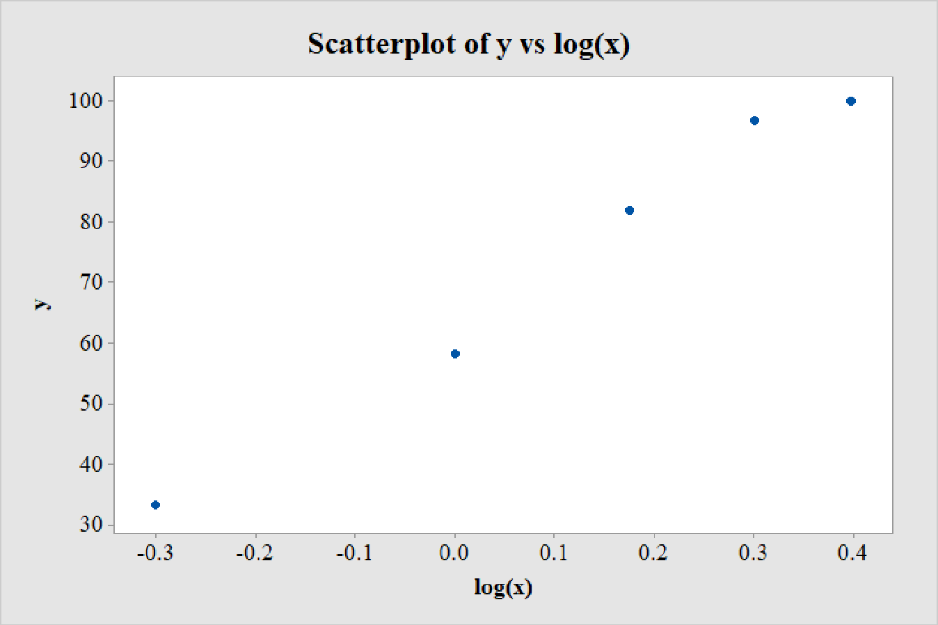
A careful observation of the scatterplot between y and
On the other hand, the scatterplot between y and
Thus, the transformation
d.
Find the least-squares regression line between y and the transformation recommended in the previous part.
d.
Answer to Problem 18CRE
The least-squares regression equation between y and the transformation recommended in the previous part, that is,
Explanation of Solution
Calculation:
The least-squares regression line can be obtained using software.
Regression:
Software procedure:
Step by step procedure to get regression equation using MINITAB software is given as,
- Choose Stat > Regression > Regression > Fit Regression Model.
- Under Responses, enter the column of y.
- Under Continuous predictors, enter the columns of log(x).
- Choose Results and select Analysis of Variance, Model Summary, Coefficients, Regression Equation.
- Click OK on all dialogue boxes.
The outputs using MINITAB software is given as follows:
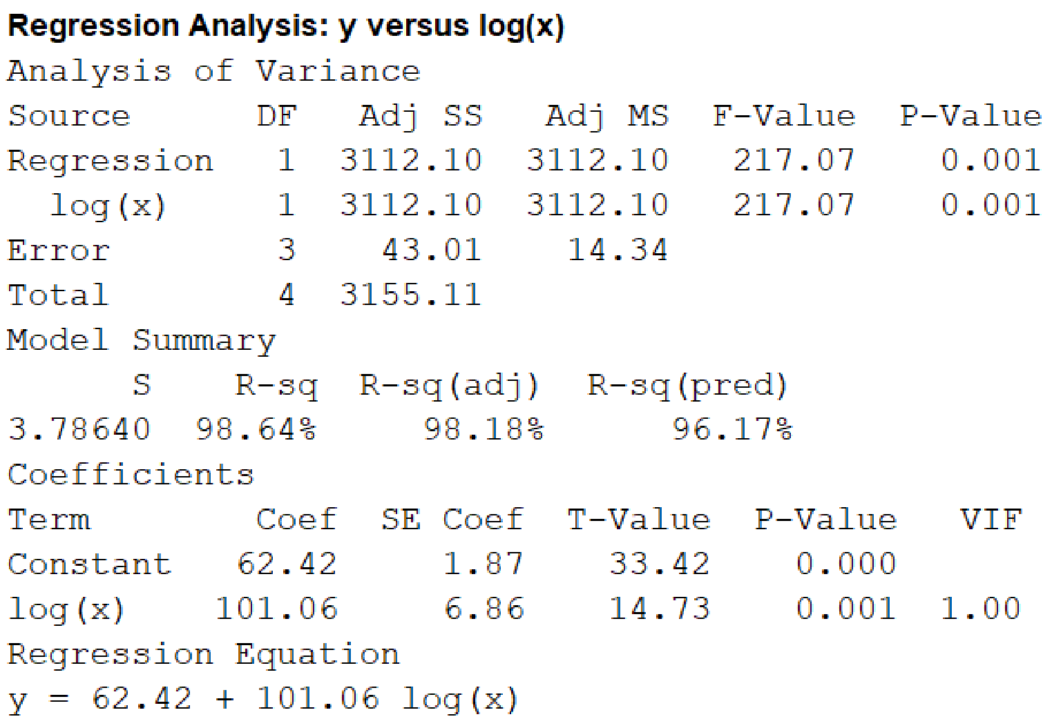
From the output, the least-squares regression equation between y and the transformation recommended in the previous part, that is,
e.
Predict the success for an energy shock 1.75 times the threshold.
Predict the success for an energy shock 0.8 times the threshold.
e.
Answer to Problem 18CRE
The success for an energy shock 1.75 times the threshold is 86.98%.
The success for an energy shock 0.8 times the threshold is 52.63%.
Explanation of Solution
Calculation:
The energy of shock is given as a multiple of the threshold of defibrillation.
For an energy shock 1.75 times the threshold,
Thus, the success for an energy shock 1.75 times the threshold is 86.98%.
For an energy shock 0.8 times the threshold,
Thus, the success for an energy shock 0.8 times the threshold is 52.63%.
Want to see more full solutions like this?
Chapter 5 Solutions
Introduction to Statistics and Data Analysis


- The article “Effect of Varying Solids Concentration and Organic Loading on the Performance of Temperature Phased Anaerobic Digestion Process” (S. Vandenburgh and T. Ellis, Water Environment Research, 2002:142–148) discusses experiments to determine the effect of the solids concentration on the performance of treatment methods for wastewater sludge. In the first experiment, the concentration of solids (in g/L) was 43.94 ± 1.18. In the second experiment, which was independent of the first, the concentration was 48.66 ± 1.76. Estimate the difference in the concentration between the two experiments, and find the uncertainty in the estimate.arrow_forwardrofessor Cornish studied rainfall cycles and sunspot cycles. (Reference: Australian Journal of Physics, Vol. 7, pp. 334-346.) Part of the data include amount of rain (in mm) for 6-day intervals. The following data give rain amounts for consecutive 6-day intervals at Adelaide, South Australia. 7 28 7 1 69 3 1 4 22 7 16 4 54 160 60 73 27 3 3 1 7 144 107 4 91 44 1 8 4 22 4 59 116 52 4 155 42 24 11 43 3 24 19 74 26 63 110 39 34 71 52 39 8 0 15 2 14 9 1 2 4 9 6 10 (i) Find the median. (Use 1 decimal place.)(ii) Convert this sequence of numbers to a sequence of symbols A and B, where A indicates a value above the median and B a value below the median. Test the sequence for randomness about the median at the 5% level of significance. (b) Find the number of runs R, n1, and n2. Let n1 = number of values above the median and n2 = number of values below the median. R n1 n2 (c) In the case, n1 > 20, we cannot use Table 10 of Appendix II to find the critical…arrow_forwardRefer to Exercise 8.S.6. Analyze these data using a Wilcoxon signed-rank test.arrow_forward
- In a typical multiple linear regression model where x1 and x2 are non-random regressors, the expected value of the response variable y given x1 and x2 is denoted by E(y | 2,, X2). Build a multiple linear regression model for E (y | *,, *2) such that the value of E(y | x1, X2) may change as the value of x2 changes but the change in the value of E(y | X1, X2) may differ in the value of x1 . How can such a potential difference be tested and estimated statistically?arrow_forwardAn article in the Journal of Applied Polymer Science (Vol. 56, pp. 471–476, 1995) studied the effect of the mole ratio of sebacic acid on the intrinsic viscosity of copolyesters.- The data follows: Viscosity 0.45 0.2 0.34 0.58 0.7 0.57 0.55 0.44 Mole ratio 1 0.9 0.8 0.7 0.6 0.5 0.4 0.3 (a) Construct a scatter diagram of the data.arrow_forwardConsider a cohort study to compare the mortality rate of myocardial infarction (MI) in men with sedentary work (exposed group) to men with physically active work (unexposed). If in the exposed, there were 36,000 person (man) years of observation and 126 deaths whereas the unexposed had 24,000 man-years of observation and 44 deaths. Compute the following a) Mortality rate in each cohort? b) What is the relative risk of dying, comparing these 2 groups? c) What is the attributable risk of sedentary work? d) What is the attributable benefit of physical activity? e) If we assume that MI is associated with the mortality in this cohort (causality), what proportion of the disease in the higher group is potentially preventable?arrow_forward
- The article in the ASCE Journal of Energy Engineering (1999, Vol. 125, pp.59-75) describes a study of the thermal inertia properties of autoclaved aerated concrete used as a building material. Five samples of the material were tested in a structure, and the average interior temperatures (°C) reported were as follows: 23.01, 22.22, 22.04, 22.62, and 22.59. Test that the average interior temperature is equal to 22.5°C using alpha (a) = 0.05. This problem is a test on what population parameter? What is the null and alternative hypothesis? What are the Significance level and type of test? What standardized test statistic will be used? What is the standard test statistic? What is the Statistical Decision? What is the statistical decision in the statement form?arrow_forwardThe Turbine Oil Oxidation Test (TOST) and the Rotating Bomb Oxidation Test (RBOT) are two different procedures for evaluating the oxidation stability of steam turbine oils. An article reported the accompanying observations on x = TOST time (hr) and y = RBOT time (min) for 12 oil specimens. TOST 4200 3600 3750 3650 4050 2770 RBOT 370 345 375 315 350 205 TOST 4870 4525 3450 2700 3750 3325 RBOT 400 380 285 220 345 290 (a) Calculate the value of the sample correlation coefficient. (Round your answer to four decimal places.) r = Carry out a test of hypotheses to decide whether RBOT Time and TOST time are linearly related. (Use ? = 0.05.) Calculate the test statistic and determine the P-value. (Round your test statistic to two decimal places and your P-value to three decimal places.) t = P-value =arrow_forwardA deficiency of the trace element selenium in the diet can negatively impact growth, immunity, muscle and neuromuscular function, and fertility. The introduction of selenium supplements to dairy cows is justified when pastures have low selenium levels. Authors of the article “Effects of Short-Term Supplementation with Selenised Yeast on Milk Production and Composition of Lactating Cows” (Australian J. of Dairy Tech., 2004: 199–203) supplied the following data on milk selenium concentration (mg/L) for a sample of cows given a selenium supplement and a control sample given no supplement, both initially and after a 9-day period. Obs Init Se Init Cont Final Se Final Cont 1 11.4 9.1 138.3 9.3 2 9.6 8.7 104 8.8 3 10.1 9.7 96.4 8.8 4 8.5 10.8 89 10.1 5 10.3 10.9 88 9.6 6 10.6 10.6 103.8 8.6 7 11.8 10.1 147.3 10.4 8 9.8 12.3 97.1 12.4 9 10.9 8.8 172.6 9.3 10 10.3…arrow_forward
- Consider the following measurements of blood hemoglobin concentrations (in g/dL) from three human populations at different geographic locations: population1 = [ 14.7 , 15.22, 15.28, 16.58, 15.10 ] population2 = [ 15.66, 15.91, 14.41, 14.73, 15.09] population3 = [ 17.12, 16.42, 16.43, 17.33] What is the standard error of the difference between the means of population 1 and population 2, needed to calculate the Tukey-Kramer q-statistic? What is the Tukey-Kramer q-statistic for populations 1 and 2? (Report the absolute value, if you get a negative number, multiply by -1)arrow_forwardSample data on weekly sales of two dairy products, X and Y were reported as follows: Lilongwe dairy, X 120 100 160 250 180 130 300 40 Long life, Y 70 86 67 100 45 80 90 95 a. Apply the CV, and find out which of the 2 products shows greater fluctuations in sales.arrow_forwardListed below are amounts of strontium-90 (in millibecquerels, or mBq) in a simple random sample of baby teeth obtained from residents in a region born after 1979. Use the given data to construct a boxplot and identify the 5-number summary. 129 132 135 140 141 145 148 151 154 157 159 159 161 164 165 170 173 173 175 182 The 5-number summary is nothing, nothing, nothing, nothing, and nothing, all in mBq. (Use ascending order. Type integers or decimals. Do not round.)arrow_forward
 Glencoe Algebra 1, Student Edition, 9780079039897...AlgebraISBN:9780079039897Author:CarterPublisher:McGraw Hill