
Concept explainers
Videos
The purpose of an Automatic Voltage Regulator is to maintain constant the voltage generated in an electrical power system, despite load and line variations, in an electrical power distribution system (Gozde, 2011). Figure P5.42 shows the block
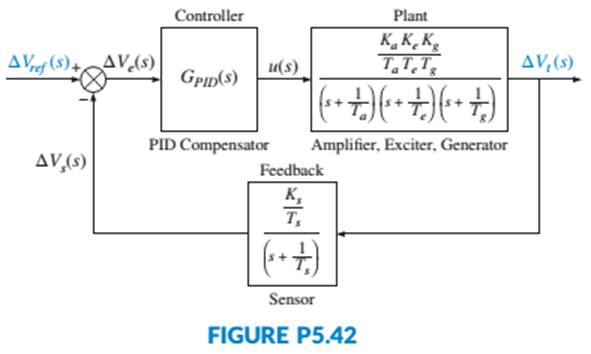
diagram of such a system. Assuming Ka= 10, Ta= 0.1, Ke= 1, Te= 0.4, Kg= 1, Tg= 1, Ks= 1, Ts= 0.001, and the controller,
Want to see the full answer?
Check out a sample textbook solution
Chapter 5 Solutions
CONTROL SYSTEMS ENGINEERING - WILEYPLUS


- 1%9• l1, ie O 10:YE Consider the system presented by the following transfer function y(s) s+2 и (s) + 2s +3 The state-space model is A = -2 C=[2 1] D=[2] а. B = b. A= B = |-3 -2 C=[1 0] D=[0] c. A = B = -3 d. A= C =[2 1] D=[0] B = -3 -2 Select one: O a. d O b. a II > IIarrow_forward2. The state-equations of the control system shown in Fig.1 is: U(s) 2 Y(s) s(s? + 3s + 12)arrow_forwardThe Gilles & Retzbach model of a distillation column, the system model includes the dynamics of a boiler, is driven by the inputs of steam flow and the flow rate of the vapour side stream, and the measurements are the temperature changes at two different locations along the column. The state space model is given by: x = 0 00 -30.3 0.00012 -6.02 0 0 0 -3.77 00 0 -2.80 0 0 Is the system?: a. unstable b. C. not unstable x+ 6.15 0 0 0 0 3.04 0 0.052 not asymptotically stable d. asymptotically stable -1 u y = 0 0 0 0 -7.3 0 0 -25.0 Xarrow_forward
- Represent the translational mechanical system shown below in state space, where x3(t) is the output. State variables ニュ=X 3 = X2 Let -4 = X2 Es = X3 E6 = X3 x1(t) x2(t) x3(t) 1 N-sim 1 N-sim 1 Nim 1 Nim 1kg 1kg 1 kg J1 J2 J3 Fit)arrow_forwardA velocity of a vehicle is required to be controlled and maintained constant even if there are disturbances because of wind, or road surface variations. The forces that are applied on the vehicle are the engine force (u), damping/resistive force (b*v) that opposing the motion, and inertial force (m*a). A simplified model is shown in the free body diagram below. From the free body diagram, the ordinary differential equation of the vehicle is: m * dv(t)/ dt + bv(t) = u (t) Where: v (m/s) is the velocity of the vehicle, b [Ns/m] is the damping coefficient, m [kg] is the vehicle mass, u [N] is the engine force. Question: Assume that the vehicle initially starts from zero velocity and zero acceleration. Then, (Note that the velocity (v) is the output and the force (w) is the input to the system): A. Use Laplace transform of the differential equation to determine the transfer function of the system.arrow_forwardA velocity of a vehicle is required to be controlled and maintained constant even if there are disturbances because of wind, or road surface variations. The forces that are applied on the vehicle are the engine force (u), damping/resistive force (b*v) that opposing the motion, and inertial force (m*a). A simplified model is shown in the free body diagram below. From the free body diagram, the ordinary differential equation of the vehicle is: m * dv(t)/ dt + bv(t) = u (t) Where: v (m/s) is the velocity of the vehicle, b [Ns/m] is the damping coefficient, m [kg] is the vehicle mass, u [N] is the engine force. Question: Assume that the vehicle initially starts from zero velocity and zero acceleration. Then, (Note that the velocity (v) is the output and the force (w) is the input to the system): 1. What is the order of this system?arrow_forward
- 6. Consider the mechanical system shown in Fig. 8. Let V(t) be the input and the acceleration of the mass be the output. Derive the state equations and the output equation using linear graphs and normal trees. B m V₁(t) Figure 8: A mechanical system with an across-variable sourcearrow_forward11. Consider a system that can be modeled as shown. The input x in (t) is a prescribed motion at the right end of spring k 2. Find X(s) the system transfer function Xeq(s)* m k₂ ww Xin The values of the parameters are m= 30 kg, k ₁=700 N/m, k 2= 1300 N/m, and b=200 N- s/m. Write a MATLAB script file that: (a) calculates the natural frequency, damping ratio, and damped natural frequency for the system; and (b) uses the impulse command to find and plot the response of the system to a unit impulse input.arrow_forward1. Verify Eqs. 1 through 5. Figure 1: mass spring damper In class, we have studied mechanical systems of this type. Here, the main results of our in-class analysis are reviewed. The dynamic behavior of this system is deter- mined from the linear second-order ordinary differential equation: where (1) where r(t) is the displacement of the mass, m is the mass, b is the damping coefficient, and k is the spring stiffness. Equations like Eq. 1 are often written in the "standard form" ď²x dt2 r(t) = = tan-1 d²r dt2 m. M +25wn +wn²x = 0 (2) The variable wn is the natural frequency of the system and is the damping ratio. If the system is underdamped, i.e. < < 1, and it has initial conditions (0) = zot-o = 0, then the solution to Eq. 2 is given by: IO √1 x(1) T₁ = +b+kr = 0 dt 2π dr. dt ل لها -(wat sin (wat +) and is the damped natural frequency. In Figure 2, the normalized plot of the response of this system reveals some useful information. Note that the amount of time Ta between peaks is…arrow_forward
- for principle of öpelaliuil. Q4: A robot is used to service (load/unload) three machines in a cell, where the three machines have the same cycle time as 50 sec. the cycle time is divided as follow: Decide how this robot should service these three machines to Machine (M) Load/Unload Run M1 25 25 optimize the machine interference. M2 15 35 M3 10 40arrow_forward28. Find the transfer function, G(s) = X1(s)/F(s), for the translational mechanical system shown in Figure P2.13. [Section: 2.5] 2 N-s/m X3(1) 2 N-s/m (1)'x- [4 kg 2 N-s/m 6 N/m 6 N/m 4 kg 0000 4 kg "Frictionless FIGURE P2.13 USE MATRIX METHODarrow_forwardFind: State-space representation Note: Output of mechanical system is X3(t) Given: M1=1 kg, M2=1 kg, M3=1 kg K1=1 N/m, K2=1 N/m Fv1=1 N-s/m, Fv2=1 N-s/m, Fv3=1 N-s/m, Fv4=1 N-s/marrow_forward
 Elements Of ElectromagneticsMechanical EngineeringISBN:9780190698614Author:Sadiku, Matthew N. O.Publisher:Oxford University Press
 Mechanics of Materials (10th Edition)Mechanical EngineeringISBN:9780134319650Author:Russell C. HibbelerPublisher:PEARSON
 Thermodynamics: An Engineering ApproachMechanical EngineeringISBN:9781259822674Author:Yunus A. Cengel Dr., Michael A. BolesPublisher:McGraw-Hill Education
 Control Systems EngineeringMechanical EngineeringISBN:9781118170519Author:Norman S. NisePublisher:WILEY
 Mechanics of Materials (MindTap Course List)Mechanical EngineeringISBN:9781337093347Author:Barry J. Goodno, James M. GerePublisher:Cengage Learning
 Engineering Mechanics: StaticsMechanical EngineeringISBN:9781118807330Author:James L. Meriam, L. G. Kraige, J. N. BoltonPublisher:WILEY