
Concept explainers
Videos
The system shown in Figure P6.16 has
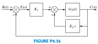
a. The value of K2for which the inner loop will have two equal negative real poles and the associated range of K1for system stability.
b. The value of K1at which the system oscillates and the associated frequency of oscillation.
c. The gain K1at which a real closed-loop pole is at
d. If the response in Part d can be approximated as a second-order response, find the %OS and settling time, Ts, when the input is a unit step, r(t) = u(t).
Want to see the full answer?
Check out a sample textbook solution
Chapter 6 Solutions
CONTROL SYSTEMS ENGINEERING


- For the control system shown in Fig. 3.16: (a) plot the root loci of the system (b) find the value of gain K such that the damping ratio of the dominant closed-loop poles is 0.5 (c) obtain all the closed-loop poles using MATLAB (d) plot the unit-step response curve using MATLAB. K Input s(s²+5s+7) Outputarrow_forwardFigure 1 shows an electrical system comprising a series RLC circuit and input voltagesource ein(t).(a) Derive the input-output equation with output y = I and input u = ein(t). (b) Using the derived input-output equation, drive the system transfer function G(s)that relates output to input. Use the following numerical values for the electrical systemparameters: resistance R = 2Ω, inductance L = 0.25H, and capacitance C = 0.4F. (c) Using the derived transfer function, derive the time-domain ordinary differentialequation for the input-output equation of this electrical system. (d) Draw the complete block diagram of this series RLC circuit using the derived transferfunction.arrow_forwardFigure Q2 shows the block diagram of a unity-feedback control system Proportional Controller Plant R(s) C(s). s(3s +1) 5+2s² +4 K 2.1- Determine the characteristic equation. 2.2- Using the Routh-Hurwitz criterion to determine the range of gain, K to ensure stability and marginally stability in the unity feedback syste m.arrow_forward
- Consider the system shown in Figure .Plot the root loci with MATLAB. Locate the closed-loop poles when the gain K is set equal to 2. K(s+1) s(s²+2s+6) Figure s+1arrow_forward1.block diagram physical meaning and the time response for different inputsarrow_forwardThe close loop system block diagram is given below .Find the transfer function of the given system. 02 G Error Harrow_forward
- A system can be approximately expressed as X₁ = −T₁×₁ +σx2 x2=-T2x2 + ku a. Given ₁ = 8,σ = 4, k = 0, find the range of T2 such that the system x = Ax is asymptotical stable. b. Given ₁ = 8, t₂ = −1, σ = k = 1, design a state-feedback controller, such that the system x = Ax+Bu is asymptotical stable. LG 11-7 IZ-N 13-arrow_forwardIt is known that G(s)= $4 and the closed-loop structure is shown below: R(s) + E(s) A (7 K(s + 2) G(s) +s C(s) Find the range of K for which the closed-loop system will have at least two right half-plane poles. (Tip: consider no zeros in 1st column of Routh table and special cases separately)arrow_forwardSelecting the new closed-loop poles in a location where the dominant closed- loop poles are located will result in state-feedback gains: s^2+4s+10arrow_forward
- 6. Consider the mechanical system shown in Fig. 8. Let V(t) be the input and the acceleration of the mass be the output. Derive the state equations and the output equation using linear graphs and normal trees. B m V₁(t) Figure 8: A mechanical system with an across-variable sourcearrow_forwardP4. The open loop transfer function of a unity feedback system is given by G (s) = K s(as+1)(Bs+1) Determine the range of K for stability in terms of a and B.arrow_forwardCalculate the poles, decay rate, damped natural frequency, undamped natural fre- quency, and damping ratio of the system represented by the transfer function below. State whether the system is overdamped, underdamped, undamped, critically damped, or unstable. G(s) = = 28² + 3s + 5 s² + 16arrow_forward
 Elements Of ElectromagneticsMechanical EngineeringISBN:9780190698614Author:Sadiku, Matthew N. O.Publisher:Oxford University Press
 Mechanics of Materials (10th Edition)Mechanical EngineeringISBN:9780134319650Author:Russell C. HibbelerPublisher:PEARSON
 Thermodynamics: An Engineering ApproachMechanical EngineeringISBN:9781259822674Author:Yunus A. Cengel Dr., Michael A. BolesPublisher:McGraw-Hill Education
 Control Systems EngineeringMechanical EngineeringISBN:9781118170519Author:Norman S. NisePublisher:WILEY
 Mechanics of Materials (MindTap Course List)Mechanical EngineeringISBN:9781337093347Author:Barry J. Goodno, James M. GerePublisher:Cengage Learning
 Engineering Mechanics: StaticsMechanical EngineeringISBN:9781118807330Author:James L. Meriam, L. G. Kraige, J. N. BoltonPublisher:WILEY