Statistics for Engineers and Scientists
4th Edition
ISBN: 9780073530789
Author: Navidi
Publisher: MCG
expand_more
expand_more
format_list_bulleted
Concept explainers
Videos
Textbook Question
Chapter 7, Problem 11SE
The article “Estimating Population Abundance in Plant Species with Dormant Life-Stages: Fire and the Endangered Plant Grevillea caleye R. Br.” (T. Auld and J. Scott, Ecological Management and Restoration, 2004:125–129) presents estimates of population sizes of a certain rare shrub in areas burnt by fire. The following table presents population counts and areas (in m2) for several patches containing the plant.
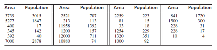
- a. Compute the least-squares line for predicting population (y) from area (x).
- b. Plot the residuals versus the fitted values. Does the model seem appropriate?
- c. Compute the least-squares line for predicting ln y from ln x.
- d. Plot the residuals versus the fitted values. Does the model seem appropriate?
- e. Using the more appropriate model, construct a 95% prediction interval for the population in a patch whose area is 3000m2.
Expert Solution & Answer
Want to see the full answer?
Check out a sample textbook solution
Students have asked these similar questions
The table below shows the numbers of bushels of barley cultivated per acre for 12 one-acre plots of land for two different strains of barley, PHT-34 and CBX-21.
PHT-34
CBX-21
43
55
49
46
47
43
38
44
47
45
45
49
50
47
46
59
46
52
46
49
45
48
43
51
Determine the minimum data value, the quartiles, and the maximum data value for the PHT-34 and CBX-21 data sets.
PHT-34
CBX-21
min
Q1
Q2
Q3
max
The following table presents the percentage of students who tested proficient in reading and the percentage who tested proficient in math for each of the ten most populous states in the United States.
State
Percent Proficient in Reading
Percent Proficient in Mathematics
California
60
59
Texas
73
78
New York
75
70
Florida
66
68
Illinois
75
70
Pennsylvania
79
77
Ohio
79
76
Michigan
73
66
Georgia
67
64
North Carolina
71
73
Compute the least-squares regression line for predicting math proficiency from reading proficiency.
Predict the math proficiency for another state with reading proficiency of 63 percent.
Is a baseball players' slugging percentage correlated to their strikeout percentage? A random sample of n=6n=6professional baseball players gave the following data (Source: baseball-reference.com)
Slugging
0.396
0.42
0.323
0.078
0.473
0.467
Strikeouts
27
14.3
30.8
47.1
17.8
36.7
Find the least squares line if we consider slugging percengtage as the explanatory variable and strikeout percentage as the response variable. (Round the y-intercept and slope to 2 decimal places.)y^ =
For a unit increase in slugging percentage, how much of a decrease Correct in strikeout percentage is predicted? (Round your answer to 2 decimal places.)
What percentage of the variation in strikeout percentage (yy) can be explained by slugging percentage (xx) and the least squares line? (Round to the nearest percent.)
p-value (Round to four decimal places)
Chapter 7 Solutions
Statistics for Engineers and Scientists
Ch. 7.1 - Compute the correlation coefficient for the...Ch. 7.1 - For each of the following data sets, explain why...Ch. 7.1 - For each of the following scatterplots, state...Ch. 7.1 - True or false, and explain briefly: a. If the...Ch. 7.1 - In a study of ground motion caused by earthquakes,...Ch. 7.1 - A chemical engineer is studying the effect of...Ch. 7.1 - Another chemical engineer is studying the same...Ch. 7.1 - Tire pressure (in kPa) was measured for the right...Ch. 7.1 - Prob. 10ECh. 7.1 - The article Drift in Posturography Systems...
Ch. 7.1 - Prob. 12ECh. 7.1 - Prob. 13ECh. 7.1 - A scatterplot contains four points: (2, 2), (1,...Ch. 7.2 - Each month for several months, the average...Ch. 7.2 - In a study of the relationship between the Brinell...Ch. 7.2 - A least-squares line is fit to a set of points. If...Ch. 7.2 - Prob. 4ECh. 7.2 - In Galtons height data (Figure 7.1, in Section...Ch. 7.2 - In a study relating the degree of warping, in mm....Ch. 7.2 - Moisture content in percent by volume (x) and...Ch. 7.2 - The following table presents shear strengths (in...Ch. 7.2 - Structural engineers use wireless sensor networks...Ch. 7.2 - The article Effect of Environmental Factors on...Ch. 7.2 - An agricultural scientist planted alfalfa on...Ch. 7.2 - Curing times in days (x) and compressive strengths...Ch. 7.2 - Prob. 13ECh. 7.2 - An engineer wants to predict the value for y when...Ch. 7.2 - A simple random sample of 100 men aged 2534...Ch. 7.2 - Prob. 16ECh. 7.3 - A chemical reaction is run 12 times, and the...Ch. 7.3 - Structural engineers use wireless sensor networks...Ch. 7.3 - Prob. 3ECh. 7.3 - Prob. 4ECh. 7.3 - Prob. 5ECh. 7.3 - Prob. 6ECh. 7.3 - The coefficient of absorption (COA) for a clay...Ch. 7.3 - Prob. 8ECh. 7.3 - Prob. 9ECh. 7.3 - Three engineers are independently estimating the...Ch. 7.3 - In the skin permeability example (Example 7.17)...Ch. 7.3 - Prob. 12ECh. 7.3 - In a study of copper bars, the relationship...Ch. 7.3 - Prob. 14ECh. 7.3 - In the following MINITAB output, some of the...Ch. 7.3 - Prob. 16ECh. 7.3 - In order to increase the production of gas wells,...Ch. 7.4 - The following output (from MINITAB) is for the...Ch. 7.4 - The processing of raw coal involves washing, in...Ch. 7.4 - To determine the effect of temperature on the...Ch. 7.4 - The depth of wetting of a soil is the depth to...Ch. 7.4 - Good forecasting and control of preconstruction...Ch. 7.4 - The article Drift in Posturography Systems...Ch. 7.4 - Prob. 7ECh. 7.4 - Prob. 8ECh. 7.4 - A windmill is used to generate direct current....Ch. 7.4 - Two radon detectors were placed in different...Ch. 7.4 - Prob. 11ECh. 7.4 - The article The Selection of Yeast Strains for the...Ch. 7.4 - Prob. 13ECh. 7.4 - The article Characteristics and Trends of River...Ch. 7.4 - Prob. 15ECh. 7.4 - The article Mechanistic-Empirical Design of...Ch. 7.4 - An engineer wants to determine the spring constant...Ch. 7 - The BeerLambert law relates the absorbance A of a...Ch. 7 - Prob. 2SECh. 7 - Prob. 3SECh. 7 - Refer to Exercise 3. a. Plot the residuals versus...Ch. 7 - Prob. 5SECh. 7 - The article Experimental Measurement of Radiative...Ch. 7 - Prob. 7SECh. 7 - Prob. 8SECh. 7 - Prob. 9SECh. 7 - Prob. 10SECh. 7 - The article Estimating Population Abundance in...Ch. 7 - A materials scientist is experimenting with a new...Ch. 7 - Monitoring the yield of a particular chemical...Ch. 7 - Prob. 14SECh. 7 - Refer to Exercise 14. Someone wants to compute a...Ch. 7 - Prob. 16SECh. 7 - Prob. 17SECh. 7 - Prob. 18SECh. 7 - Prob. 19SECh. 7 - Use Equation (7.34) (page 545) to show that 1=1.Ch. 7 - Use Equation (7.35) (page 545) to show that 0=0.Ch. 7 - Prob. 22SECh. 7 - Use Equation (7.35) (page 545) to derive the...
Additional Math Textbook Solutions
Find more solutions based on key concepts
A father rates his daughter as a 2 on a 7-point scale (from 1 to 7) of crankiness. In this example, (a) what is...
Statistics for Psychology
Compare and contrast the nonscientific methods for knowing or acquiring knowledge (tenacity, intuition, authori...
Research Methods for the Behavioral Sciences (MindTap Course List)
z Scores. In Exercises 5-8, express all z scores with two decimal places.
8. Plastic Waste Data Set 31 “Garbage...
Elementary Statistics Using Excel (6th Edition)
Provide an example of a qualitative variable and an example of a quantitative variable.
Elementary Statistics (Text Only)
TRY IT YOURSELF 2
Determine whether each number describes a population parameter or a sample statistic. Explain...
Elementary Statistics: Picturing the World (7th Edition)
In a test of the quality of two television commercials, each commercial was shown in a separate test area six t...
Statistics for Business & Economics, Revised (MindTap Course List)
Knowledge Booster


Learn more about
Need a deep-dive on the concept behind this application? Look no further. Learn more about this topic, statistics and related others by exploring similar questions and additional content below.Similar questions
- From the below table, Use excels to find the answer for the below questions: State Percentage Proficient in Reading Percentage Proficient in Mathematics California 60 59 Texas 73 78 New York 75 70 Florida 66 68 Illinois 75 70 Pennsylvania 79 77 Ohio 79 76 Michigan 73 66 Georgia 67 64 North Carolina 71 73 Activities: Compute the least-squares regression line for predicting math proficiency from reading proficiency. Interpretation of the least-squares regression line in part a.arrow_forwardThe following table shows how many weeks a sample of 6 persons have worked at an automobile inspection station and on any given day: a) Find the least squares estimators and the values for a and b ??? = ___________ ? = ___________ ??? = ___________ ? = ___________ ??? = ___________ b) Determine AND WRITE the equation for the best fit line. c) Find the correlation coefficient, r, and describe the relationship between weeks in the program and time improvement.arrow_forwardA sociologist is interested in the relation between x = number of job changes and y = annual salary (in thousands of dollars) for people living in the Nashville area. A random sample of 10 people employed in Nashville provided the following information. x (number of job changes) 5 3 6 6 1 5 9 10 10 3 y (Salary in $1000) 36 37 34 32 32 38 43 37 40 33 (d) If someone had x = 2 job changes, what does the least-squares line predict for y, the annual salary? (Round your answer to two decimal places.)thousand dollars thousand dollarsarrow_forward
- Consider a cohort study to compare the mortality rate of myocardial infarction (MI) in men with sedentary work (exposed group) to men with physically active work (unexposed). If in the exposed, there were 36,000 person (man) years of observation and 126 deaths whereas the unexposed had 24,000 man-years of observation and 44 deaths. Compute the following a) Mortality rate in each cohort? b) What is the relative risk of dying, comparing these 2 groups? c) What is the attributable risk of sedentary work? d) What is the attributable benefit of physical activity? e) If we assume that MI is associated with the mortality in this cohort (causality), what proportion of the disease in the higher group is potentially preventable?arrow_forwardHere is a dataset containing plant growth measurements of plants grown in solutions of commonly-found chemicals in roadway runoff.Phragmites australis, a fast-growing non-native grass common to roadsides and disturbed wetlands of Tidewater Virginia, was grown in a greenhouse and watered with either: Distilled water (control); A weak petroleum solution (representing standard roadway runoff); Sodium chloride solution; Magnesium chloride solution; De-icing brine (50% sodium chloride and 50% magnesium chloride).Twenty grass preparations were used for each solution, and total growth (in cm) was recorded after watering every other day for 40 days.-Perform the correct statistical test to determine the p-value.-Report your answer rounded to four decimal places.-You should use formulas, functions, and the Data Analysis ToolPak in MS Excel to avoid additive rounding errors. Here are some useful functions: =t.test(array1,array2,tails,type) Produces a p-value for any…arrow_forwardThe following summary statistics resulted from a study of the relationship between the cost ofa barrel of crude oil (x) and the price of a gallon of regular unleaded gasoline (y).n = 12x 241.1 y 14.34 4,932.82 x 17.288 2 y xy 291.55(1) Compute the sample correlation r and use it to judge the strength of linear relationshipbetween x and y.(2) Obtain the equation of the least squares line, and interpret its slope and intercept.(3) Predict the price of a gallon of regular unleaded gasoline when the cost of a barrel of crudeoil is 50.arrow_forward
- The following table presents the ages of 8 U.S. presidents and their wives on the first day of their presidencies. Name Her Age His Age Barack and Michelle Obama 45 47 George W. and Laura Bush 54 54 Bill and Hillary Clinton 45 46 Ronald and Nancy Reagan 55 64 Gerald and Betty Ford 59 69 Lyndon and Lady Bird Johnson 56 61 John and Jacqueline Kennedy 31 43 Dwight and Mamie Eisenhower 50 55 Part 1 of 4 (a) Compute the least-squares regression line for predicting the president's age from the first lady's age. Round the slope and y -intercept values to at least four decimal places. Regression line equation: =y .arrow_forwardAn automotive engineer is investigating two different types of metering devices for an electronic fuel injection system to determine whether they differ in their fuel mileage performance. The system is installed on 10 different cars, and a test is run with each metering device on each car. The data is provided below: Metering Device Car 1 2 1 17.6 16.8 2 19.4 20.0 3 18.2 17.6 4 17.1 16.4 5 15.3 16.0 6 15.9 15.9 7 16.3 16.5 8 18.0 18.4 9 17.3 16.4 10 19.1 20.1 Is there a significant difference between the means of the two metering devices? Use . Interpret the result in the context of the problem. An article in the journal Hazardous Waste and Hazardous Materials (Vol. 6, 1989) reported the results of an analysis of the weight of calcium in standard cement and cement doped with lead. Reduced levels of calcium would indicate that the hydration mechanism in the cement is blocked…arrow_forwardJensen Tire & Auto is in the process of deciding whether to purchase a maintenance contract for its new computer wheel alignment and balancing machine. Managers feel that maintenance expense should be related to usage, and they collected the following information on weekly usage (hours) and annual maintenance expense (in hundreds of dollars). Weekly Usage(hours) AnnualMaintenanceExpense 13 17.0 10 22.0 20 30.0 28 37.0 32 47.0 17 30.5 24 32.5 31 39.0 40 51.5 38 40.0 test statistic is 6.90 Find the p-value. (Round your answer to three decimal places.) p-value = State your conclusion. Reject H0. We conclude that the relationship between weekly usage (hours) and annual maintenance expense (in hundreds of dollars) is significant. Do not reject H0. We conclude that the relationship between weekly usage (hours) and annual maintenance expense (in hundreds of dollars) is significant. Reject H0. We cannot conclude that the relationship between weekly usage…arrow_forward
- A paper investigated the driving behavior of teenagers by observing their vehicles as they left a high school parking lot and then again at a site approximately 1 2 mile from the school. Assume that it is reasonable to regard the teen drivers in this study as representative of the population of teen drivers. MaleDriver FemaleDriver 1.4 -0.2 1.2 0.5 0.9 1.1 2.1 0.7 0.7 1.1 1.3 1.2 3 0.1 1.3 0.9 0.6 0.5 2.1 0.5 (a) Use a .01 level of significance for any hypothesis tests. Data consistent with summary quantities appearing in the paper are given in the table. The measurements represent the difference between the observed vehicle speed and the posted speed limit (in miles per hour) for a sample of male teenage drivers and a sample of female teenage drivers. (Use ?males − ?females. Round your test statistic to two decimal places. Round your degrees of freedom down to the nearest whole number. Round your p-value to three decimal places.) t = df =…arrow_forwardA paper investigated the driving behavior of teenagers by observing their vehicles as they left a high school parking lot and then again at a site approximately 1 2 mile from the school. Assume that it is reasonable to regard the teen drivers in this study as representative of the population of teen drivers. MaleDriver FemaleDriver 1.3 -0.3 1.3 0.6 0.9 1.1 2.1 0.7 0.7 1.1 1.3 1.2 3 0.1 1.3 0.9 0.6 0.5 2.1 0.5 (a) Use a .01 level of significance for any hypothesis tests. Data consistent with summary quantities appearing in the paper are given in the table. The measurements represent the difference between the observed vehicle speed and the posted speed limit (in miles per hour) for a sample of male teenage drivers and a sample of female teenage drivers. (Use ?males − ?females. Round your test statistic to two decimal places. Round your degrees of freedom down to the nearest whole number. Round your p-value to three decimal places.) t = df =…arrow_forward1. An article included a summary of findings regarding the use of SAT I scores, SAT II scores, and high school grade point average (GPA) to predict first-year college GPA. The article states that "among these, SAT II scores are the best predictor, explaining 17 percent of the variance in first-year college grades. GPA was second at 15.3 percent, and SAT I was last at 13.6 percent." If the data from this study were used to fit a least squares line with y = first-year college GPA and x = high school GPA, what would the value of r2 have been? r2 =_______ 2. A study was carried out to investigate the relationship between the hardness of molded plastic (y, in Brinell units) and the amount of time elapsed since the plastic was molded (x, in hours). Summary quantities include n = 15, SSResid = 1,237.628, and SSTo = 24,619.737. Calculate and interpret the coefficient of determination. (Round the coefficient of determination to four decimal places when written as a decimal and 2 decimal…arrow_forward
arrow_back_ios
SEE MORE QUESTIONS
arrow_forward_ios
Recommended textbooks for you
 Linear Algebra: A Modern IntroductionAlgebraISBN:9781285463247Author:David PoolePublisher:Cengage Learning
Linear Algebra: A Modern Introduction
Algebra
ISBN:9781285463247
Author:David Poole
Publisher:Cengage Learning
The Shape of Data: Distributions: Crash Course Statistics #7; Author: CrashCourse;https://www.youtube.com/watch?v=bPFNxD3Yg6U;License: Standard YouTube License, CC-BY
Shape, Center, and Spread - Module 20.2 (Part 1); Author: Mrmathblog;https://www.youtube.com/watch?v=COaid7O_Gag;License: Standard YouTube License, CC-BY
Shape, Center and Spread; Author: Emily Murdock;https://www.youtube.com/watch?v=_YyW0DSCzpM;License: Standard Youtube License