Concept explainers
Videos
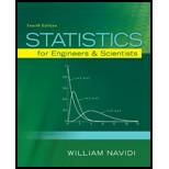
In a simulation of 30 mobile computer networks, the average speed, pause time, and number of neighbor were measured. A “neighbor” is a computer within the transmission
- a. Fit the model with Neighbors as the dependent variable, and independent variables Speed, Pause, Speed,·Pause, Speed2, and Pause2.
- b. Construct a reduced model by dropping any variables whose P-values are large, and test the plausibility of the model with an F test.
- c. Plot the residuals versus the fitted values for the reduced model. Are there any indications that the model is inappropriate? If so, what are they?
- d. Someone suggests that a model containing Pause and Pause2 as the only dependent variables is adequate. Do you agree? Why or why not?
- e. Using a best subsets software package, find the two models with the highest R2 value for each model size from one to five variables. Compute Cp and adjusted R2 for each model.
- f. Which model is selected by minimum Cp? By adjusted R2? Are they the same?
a.
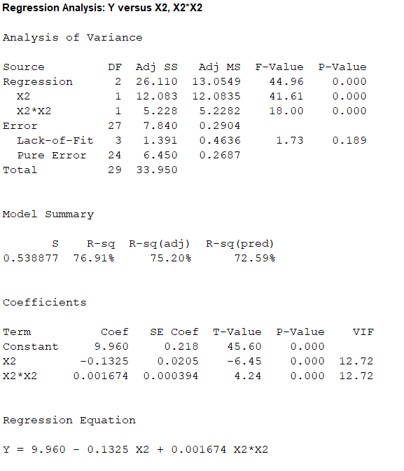
Construct a multiple linear regression model with neighbor as the dependent variable, speed, pause,
Answer to Problem 5SE
A multiple linear regression model for the given data is:
Explanation of Solution
Calculation:
The data represents the values of the variables number of neighbors, average speed and pause time for a simulation of 30 mobile network computers.
Multiple linear regression model:
A multiple linear regression model is given as
Let
Regression:
Software procedure:
Step by step procedure to obtain regression using MINITAB software is given as,
- Choose Stat > Regression > General Regression.
- In Response, enter the numeric column containing the response data Y.
- In Model, enter the numeric column containing the predictor variables X1, X2, X1*X2, X1*X1 and X2*X2.
- Click OK.
Output obtained from MINITAB is given below:
The ‘Coefficient’ column of the regression analysis MINITAB output gives the slopes corresponding to the respective variables stored in the column ‘Term’.
A careful inspection of the output shows that the fitted model is:
Hence, the multiple linear regression model for the given data is:
b.
Construct a reduced model by dropping the variables with large P- values.
Check whether the reduced model is plausible or not.
Answer to Problem 5SE
A multiple linear regression model for the given data is:
Yes, there is enough evidence to conclude that the reduced model is plausible.
Explanation of Solution
Calculation:
From part (a), it can be seen that the ‘P’ column of the regression analysis MINITAB output gives the slopes corresponding to the respective variables stored in the column ‘Term’.
By observing the P- values of the MINITAB output, it is clear that the largest P-value is 0.390 corresponding to the predictor variable
Now, the new regression has to be fitted after dropping the predictor variable
Regression:
Software procedure:
Step by step procedure to obtain regression using MINITAB software is given as,
- Choose Stat > Regression > General Regression.
- In Response, enter the numeric column containing the response data Y.
- In Model, enter the numeric column containing the predictor variables X1, X2, X1*X1 and X2*X2.
- Click OK.
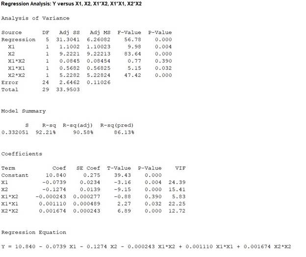
Output obtained from MINITAB is given below:
The ‘Coefficient’ column of the regression analysis MINITAB output gives the slopes corresponding to the respective variables stored in the column ‘Term’.
A careful inspection of the output shows that the fitted model is:
Hence, the multiple linear regression model for the given data is:
The full model is,
The reduced model is,
The test hypotheses are given below:
Null hypothesis:
That is, the dropped predictor of the full model is not significant to predict y.
Alternative hypothesis:
That is, the dropped predictor of the full model is significant to predict y.
Test statistic:
Where,
n represents the total number of observations.
p represents the number of predictors on the full model.
k represents the number of predictors on the reduced model.
From the obtained MINITAB outputs, the value of error sum of squares for full model is
The total number of observations is
Number of predictors on the full model is
Degrees of freedom of F-statistic for reduced model:
In a reduced multiple linear regression analysis, the F-statistic is
In the ratio, the numerator is obtained by dividing the quantity
Thus, the degrees of freedom for the F-statistic in a reduced multiple regression analysis are
Hence, the numerator degrees of freedom is
Test statistic under null hypothesis:
Under the null hypothesis, the test statistic is obtained as follows:
Thus, the test statistic is
Since, the level of significance is not specified. The prior level of significance
P-value:
Software procedure:
- Choose Graph > Probability Distribution Plot choose View Probability > OK.
- From Distribution, choose F, enter 1 in numerator df and 24 in denominator df.
- Click the Shaded Area tab.
- Choose X-Value and Right Tail for the region of the curve to shade.
- Enter the X-value as 0.76638.
- Click OK.
Output obtained from MINITAB is given below:
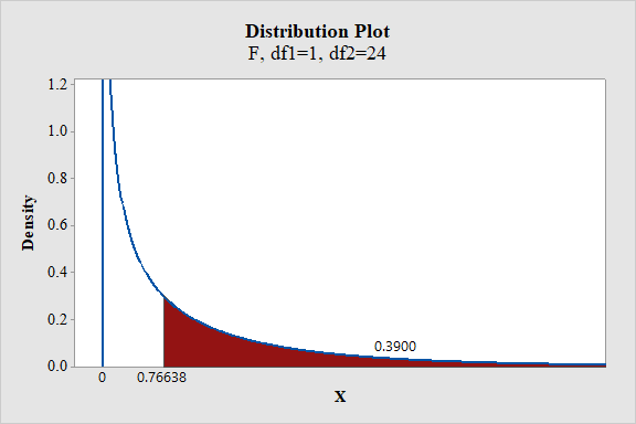
From the output, the P- value is 0.39.
Thus, the P- value is 0.39.
Decision criteria based on P-value approach:
If
If
Conclusion:
The P-value is 0.39 and
Here, P-value is greater than the
That is
By the rejection rule, fail to reject the null hypothesis.
Hence, there is sufficient evidence to conclude that the dropped predictor variable is not significant to predict the response variable y.
Thus, the reduced model is useful than the full model to predict the response variable y.
c.
Plot the residuals versus fitted line plot for the reduced model.
Check whether the model is appropriate.
Answer to Problem 5SE
Residual plot:
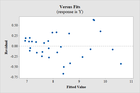
Yes, the model seems to be appropriate.
Explanation of Solution
Calculation:
Residual plot:
Software procedure:
Step by step procedure to obtain regression using MINITAB software is given as,
- Choose Stat > Regression > General Regression.
- In Response, enter the numeric column containing the response data Y.
- In Model, enter the numeric column containing the predictor variables X1, X2, X1*X1 and X2*X2.
- In Graphs, Under Residuals for plots, select Regular.
- Under Residual plots select box Residuals versus fits.
- Click OK.
Conditions for the appropriateness of regression model using the residual plot:
- The plot of the residuals vs. fitted values should fall roughly in a horizontal band contended and symmetric about x-axis. That is, the residuals of the data should not represent any bend.
- The plot of residuals should not contain any outliers.
- The residuals have to be scattered randomly around “0” with constant variability among for all the residuals. That is, the spread should be consistent.
Interpretation:
In residual plot there is high bend or pattern, which can violate the straight line condition and there is change in the spread of the residuals from one part to another part of the plot.
However, it is difficult to determine about the violation of the assumptions without the data.
Thus, the model seems to be appropriate.
d.
Check whether the model with only two dependent variables
Answer to Problem 5SE
No, the model with only two dependent variables
Explanation of Solution
Calculation:
Regression:
Software procedure:
Step by step procedure to obtain regression using MINITAB software is given as,
- Choose Stat > Regression > General Regression.
- In Response, enter the numeric column containing the response data Y.
- In Model, enter the numeric column containing the predictor variables X2 and X2*X2.
- Click OK.
Output obtained from MINITAB is given below:
The ‘Coefficient’ column of the regression analysis MINITAB output gives the slopes corresponding to the respective variables stored in the column ‘Term’.
A careful inspection of the output shows that the fitted model is:
Hence, the multiple linear regression model for the given data is:
The full model is,
The reduced model is,
The test hypotheses are given below:
Null hypothesis:
That is, the dropped predictors of the full model are not significant to predict y.
Alternative hypothesis:
That is, at least one of the dropped predictors of the full model are significant to predict y.
Test statistic:
Where,
n represents the total number of observations.
p represents the number of predictors on the full model.
k represents the number of predictors on the reduced model.
From the obtained MINITAB outputs, the value of error sum of squares for full model is
The total number of observations is
Number of predictors on the full model is
Degrees of freedom of F-statistic for reduced model:
In a reduced multiple linear regression analysis, the F-statistic is
In the ratio, the numerator is obtained by dividing the quantity
Thus, the degrees of freedom for the F-statistic in a reduced multiple regression analysis are
Hence, the numerator degrees of freedom is
Test statistic under null hypothesis:
Under the null hypothesis, the test statistic is obtained as follows:
Thus, the test statistic is
Since, the level of significance is not specified. The prior level of significance
P-value:
Software procedure:
- Choose Graph > Probability Distribution Plot choose View Probability > OK.
- From Distribution, choose F, enter 3 in numerator df and 24 in denominator df.
- Click the Shaded Area tab.
- Choose X-Value and Right Tail for the region of the curve to shade.
- Enter the X-value as 15.702.
- Click OK.
Output obtained from MINITAB is given below:
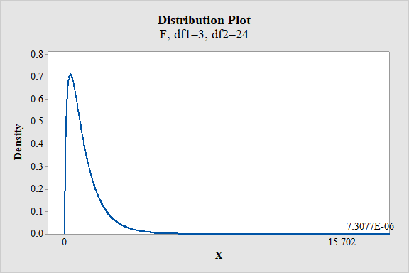
From the output, the P- value is
Thus, the P- value is
Decision criteria based on P-value approach:
If
If
Conclusion:
The P-value is
Here, P-value is less than the
That is
By the rejection rule, reject the null hypothesis.
Hence, there is sufficient evidence to conclude that at least one of the dropped predictors of the full model are significant to predict y.
Thus, the model with only two dependent variables
e.
Find the two models with the highest
Obtain the values of mallows
Answer to Problem 5SE
The two models with the highest
First model with
The values of M Mallows’
| Predictor variables | Mallows’ | Adjusted |
| 92.5 | 60.1 | |
| 97 | 58.6 | |
| 47.1 | 75.2 | |
| 53.3 | 73 | |
| 7.9 | 89.2 | |
| 15.5 | 86.4 | |
| 4.8 | 90.7 | |
| 9.2 | 89 | |
| 6 | 90.6 |
Explanation of Solution
Calculation:
Coefficient of multiple determination
The coefficient of multiple determination,
The subset with larger
Regression:
Software procedure:
Step by step procedure to obtain regression using MINITAB software is given as,
- Choose Stat > Regression > Regression> Best subsets.
- In Response, enter the numeric column containing the response data Y.
- In Model, enter the numeric column containing the predictor variables X1, X2, X1*X2, X1*X1 and X2*X2.
- Click OK.
Output obtained from MINITAB is given below:
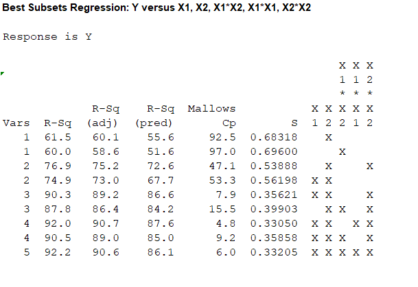
For the one predictor case, the highest value of
For the two predictor case, the highest value of
For the three predictor case, the highest value of
For the four predictor case, the highest value of
For the five predictor case, the value of
The value of
Thus, depending upon the factors affecting the analysis it would be most preferable to use the regression equation corresponding to the predictors
The second highest value of
That is, 90.6 and 90.3 are not much distinct.
Therefore, the model with
Thus, the two best models are:
First model with
From the accompanying MINITAB output, the values of Mallows’
| Predictor variables | Mallows’ | Adjusted |
| 92.5 | 60.1 | |
| 97 | 58.6 | |
| 47.1 | 75.2 | |
| 53.3 | 73 | |
| 7.9 | 89.2 | |
| 15.5 | 86.4 | |
| 4.8 | 90.7 | |
| 9.2 | 89 | |
| 6 | 90.6 |
f.
Select the variables for the model, using the Mallows’
Check whether both the models are same.
Answer to Problem 5SE
The variables for the model using the Mallows’
The variables for the model using the adjusted-
Yes, both the models are same.
Explanation of Solution
Mallows’
An important utility of the Mallows’
Mallows’
The predictor with the lowest value of
From part (e), the values of Mallows’
| Predictor variables | Mallows’ | Adjusted |
| 92.5 | 60.1 | |
| 97 | 58.6 | |
| 47.1 | 75.2 | |
| 53.3 | 73 | |
| 7.9 | 89.2 | |
| 15.5 | 86.4 | |
| 4.8 | 90.7 | |
| 9.2 | 89 | |
| 6 | 90.6 |
For the one predictor case, the lowest value of
For the two predictor case, the lowest value of
For the three predictor case, the lowest value of
For the four predictor case, the lowest value of
For the five predictor case, the value of
The value of
Thus, depending upon the factors affecting the analysis it would be most preferable to use the regression equation corresponding to the predictors
Hence, the variables for the model using the Mallows’
Adjusted
An important utility of the adjusted coefficient of multiple determination or
The adjusted coefficient of multiple determination,
For the one predictor case, the highest value of
For the two predictor case, the highest value of
For the three predictor case, the highest value of
For the four predictor case, the highest value of
For the five predictor case, the value of
The value of adjusted
Thus, provided other factors do not affect the analysis it could be most preferable to use the regression equation corresponding to the predictors,
Hence, the variables for the model using the adjusted-
Both Mallows’
Want to see more full solutions like this?
Chapter 8 Solutions
Statistics for Engineers and Scientists (Looseleaf)
Additional Math Textbook Solutions
Introductory Statistics (10th Edition)
Elementary Statistics Using the TI-83/84 Plus Calculator, Books a la Carte Edition (4th Edition)
Business Statistics: A First Course (7th Edition)
Essentials of Statistics (6th Edition)
Introductory Statistics
STATISTICS F/BUSINESS+ECONOMICS-TEXT


- To achieve the suggested power of 0.80 in MANOVA when assessing medium effect sizes in a 5 group design comprised of six dependent variables, the researcher must include at least _______ subjects per group? A) 82 B) 74 C) 90 D) 105arrow_forwardA study was undertaken to determine whether there was a significant weight (in lb) loss after one year course of therapy for diabetes, and whether the amount of weight (in lb) loss was related to initial weight. The following table gives the initial weight (x) and weight after one year of therapy (y) for 16 newly diagnosed adult diabetic patients.arrow_forwardUse this data and create a model that estimates a student's giving rate as an alumni based on the three parameters provided. If a class has a graduation rate of 74, the % of classes under 20 student equal to 55, and a Student=Faculty Ratio of 19, what should we expect our Alumni Giving Rate to be? (Enter a whole number) University Graduation Rate % of Classes Under 20 Student-Faculty Ratio Alumni Giving Rate Boston College 85 39 13 25 Brandeis University 79 68 8 33 Brown University 93 60 8 40 California Institute of Technology 85 65 3 46 Carnegie Mellon University 75 67 10 28 Case Western Reserve Univ. 72 52 8 31 College of William and Mary 89 45 12 27 Columbia University 90 69 7 31 Cornell University 91 72 13 35 Dartmouth College 94 61 10 53 Duke University 92 68 8 45 Emory University 84 65 7 37 Georgetown University 91 54 10 29 Harvard University 97 73 8 46 Johns Hopkins University 89 64 9 27 Lehigh University 81 55 11 40 Massachusetts Inst.…arrow_forward
- Which of the independent variables retains the strongest association with the number of children a respondent has when all other variables in the model are controlled?arrow_forwardRefer to the following data set. Data for Eight Phones Brand Model Price ($) Overall Score Voice Quality Talk Time (Hours) AT&T CL84100 50 73 Excellent 7 AT&T TL92271 70 70 Very Good 7 Panasonic 4773B 100 78 Very Good 13 Panasonic 6592T 80 72 Very Good 13 Uniden D2997 55 70 Very Good 10 Uniden D 1788 70 73 Very Good 7 Vtech DS6521 70 72 Excellent 7 Vtech CS6649 40 72 Very Good 7 (a) What is the average price for the phones? (Round your answer to the nearest cent.) $ Incorrect: Your answer is incorrect. (b) What is the average talk time for the phones? Incorrect: Your answer is incorrect. hoursarrow_forwardWhile it is known from data on national sales that 25% of cars sold are sedans, a survey in one city indicated that 21% of individuals owned one. Identify which of the numbers is a parameter and which is a statistic.arrow_forward
- Twenty-one mature flowers of a particular species were dissected, and the number of stamens and carpels present in each flower were counted. x, Stamens 52 68 70 38 61 51 56 65 43 37 36 74 38 35 45 72 59 60 73 76 68 y, Carpels 19 30 27 19 18 30 29 29 18 26 23 28 27 26 28 22 36 28 32 36 35 (a) Is there sufficient evidence to claim a linear relationship between these two variables at ? = .05?______(i) Find r. (Give your answer correct to three decimal places.)______(iii) State the appropriate conclusion. Reject the null hypothesis, there is not significant evidence to claim a linear relationship.Reject the null hypothesis, there is significant evidence to claim a linear relationship. Fail to reject the null hypothesis, there is significant evidence to claim a linear relationship.Fail to reject the null hypothesis, there is not significant evidence to claim a linear relationship. (b) What is the relationship between the number of stamens and the number of carpels in this…arrow_forwardThe director of a local Tourism Authority would like to know whether a family’s annual expenditure on recreation (y), measured in $000s, is related to their annual income (x), also measured in $000s. In order to explore this potential relationship, the variables x and y were recorded for 10 randomly selected families that visited the area last year. The results were as follows: Week 1 2 3 4 5 6 7 8 9 10 x 41.2 50.1 52.0 62.0 44.5 37.7 73.5 37.5 56.7 65.2 y 2.4 2.7 2.8 8.0 3.1 2.1 12.1 2.0 3.9 8.9 The summary statistics for these data are: Sum of x data: 520.4 Sum of the squares of x data: 28431.42 Sum of y data: 48 Sum of the squares of y data: 343.74 Sum of the products of x and y data: 2858.63 (i) Draw a scatter diagram of these data.arrow_forwardBecause the data in this chart are displayed as a line with no data point markers, this indicates that the dependent variable data are A) Measured (or Empirical), Numeric B) Theoretical (or Calculated), Numeric C) Measured (or Empirical), Categorical D) Theoretical (or Calculated), Categoricalarrow_forward
- The manager of an auto dealership would like to develop a model the fuel consumption of various car models based on engine size. The data is presented below. Manufacturer Engine Size (litre) Fuel Consumption (litres/100km,city driving) Hyundai Accent 1.5 8.9 Toyota Echo 1.5 7.1 Hyundai Accent 1.6 8.9 Kia rio 1.6 9.3 Mazda Protege 1.6 9.3 Honda Civic 1.7 8.1 Kia Spectra 1.8 10.9 Nissan Sentra 1.8 8.3 Pontiac Vibe 1.8 8.3 Toyota Corolla 1.8 8.1 Dodge SX 2.0 2 9.3 Ford Focus 2 8.9 Hyundai Elantra 2 9.6 Mazda Protege/proteges 2 9.9 Mitsubishi Lancer 2 9.7 Suzuki Aerio 2 9.1 Volkswagen Golf 2 10.1 Volkswagen Jetta 2 10.1 Chevrolet Cavalier 2.2 10 Oldsmobile Alero 2.2 10.1 Pontiac Grand AM 2.2 10 Saturn Ion 2.2 9.9 Saturn L200 2.2 10.1 Chrysler Sebring 2.4 10.6 Honda Accord 2.4 9.6 Hyundai Sonata 2.4 10.9 Kia Magentis 2.4 10.9 Mitsubishi Galant 2.4 11.3 Toyota Camry 2.4 10.2 Nissan Altima 2.5 10.4 Nissan Sentra 2.5 10.4…arrow_forwardThe following table was generated from the sample data of 10 junior high students regarding the average number of hours they are unsupervised per night, the average number of hours they play video games per night, and their final grades in their math class. The dependent variable is the final grade, the first independent variable (x1) is the number of hours unsupervised each night, and the second independent variable (x2) is the number of hours of video games each night. Intercept 52.536016 9.353956 5.616449 0.000802 Hours Unsupervised 7.173889 1.656518 4.330703 0.003435 Hours Playing Video Games 2.025042 1.731352 1.169631 0.280429 Step 1 of 2:Write the multiple regression equation for the computer output given. Round your answers to three decimal places. Step 2 of 2:Indicate if any of the independent variables could be eliminated at the 0.010.01 level of significance. (x1, x2, or keep all variables)arrow_forwardTwenty-one mature flowers of a particular species were dissected, and the number of stamens and carpels present in each flower were counted. x, Stamens 52 68 70 38 61 51 56 65 43 37 36 74 38 35 45 72 59 60 73 76 68 y, Carpels 21 30 29 19 20 30 29 31 20 24 21 28 27 24 28 22 34 28 32 34 35 (a) Is there sufficient evidence to claim a linear relationship between these two variables at ? = .05?(i) Find r. (Give your answer correct to three decimal places.) (b) What is the relationship between the number of stamens and the number of carpels in this variety of flower?. (Give your answers correct to two decimal places.) Y= _________ +__________ xarrow_forward
 Linear Algebra: A Modern IntroductionAlgebraISBN:9781285463247Author:David PoolePublisher:Cengage Learning