Videos
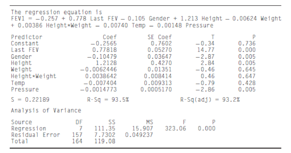
(Continues Exercise 7 in Section 8.1.) To try to improve the prediction of FEV1, additional independent variables are included in the model. These new variables are Weight (in kg), the product (interaction) of Height and Weight, and the ambient temperature (in °C). The following MINITAB output presents results of fitting the model
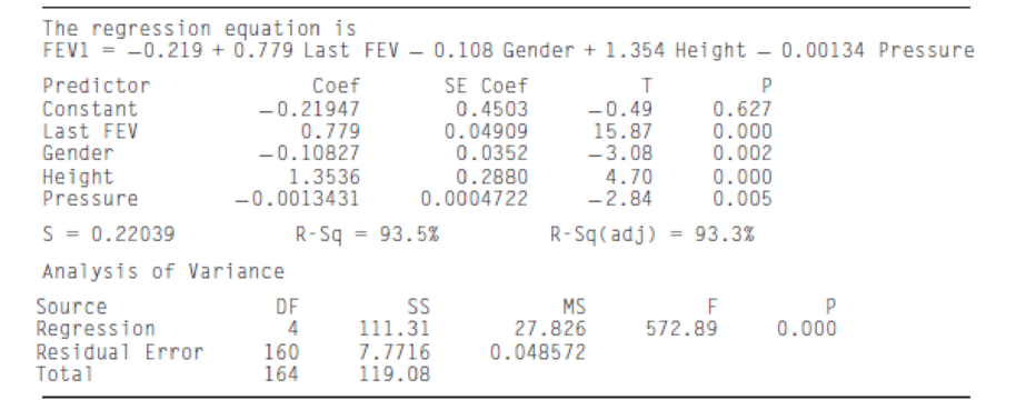
- a. The following MINITAB output, reproduced from Exercise 7 in Section 8.1, is for a reduced model in which Weight, Height·Weight, and Temp have been dropped. Compute the F statistic for testing the plausibility of the reduced model.
- b. How many degrees of freedom does the F statistic have?
- c. Find the P-value for the F statistic. Is the reduced model plausible?
- d. Someone claims that since each of the variables being dropped had large P-values, the reduced model must be plausible, and it was not necessary to perform an F test. Is this correct? Explain why or why not.
Want to see the full answer?
Check out a sample textbook solution
Chapter 8 Solutions
STATISTICS FOR ENGR.+SCI.(LL)-W/ACCESS
Additional Math Textbook Solutions
Essentials of Statistics (6th Edition)
Fundamentals of Statistics (5th Edition)
Statistics for Business & Economics, Revised (MindTap Course List)
Introduction to Statistical Quality Control
Statistical Techniques in Business and Economics


- The accompanying data file contains 40 observations on the response variable y along with the predictor variables x1 and x2. Use the holdout method to compare the predictability of the linear model with the exponential model using the first 30 observations for training and the remaining 10 observations for validation. y x1 x2 533.86 20 30 104.84 15 20 64.89 20 23 159.61 16 21 43.06 13 16 4.27 13 13 736.56 15 30 64.89 20 23 10.64 20 22 76.90 18 20 4.89 11 13 80.90 11 16 224.17 12 19 45.75 16 25 8.13 17 17 319.97 13 30 48.61 19 25 564.67 12 27 111.87 11 25 152.39 13 24 13.34 18 14 28.80 15 22 37.56 13 15 105.62 17 26 44.05 18 21 451.65 17 28 10.34 18 21 32.70 12 13 19.21 14 12 14.02 15 16 2.45 16 12 2.48 20 15 50.34 17 21 29.31 17 20 33.75 16 12 196.28 17 29 943.12 13 30 7.25 10 12 89.73 15 25 32.91 12 18 1. Use the training set to estimate Models 1 and 2. Note: Negative values should be indicated by a…arrow_forwardFor the horseshoe crab data with width, color, and spine as predictors, suppose you start a backward elimination process with the most complex model possible. Denoted by C ∗ S ∗ W, it uses main effects for each term as well as the three two-factor interactions and the three-factor interaction. Table 5.9 shows the fit for this model and various simpler models d.Finally, compare the working model at this stage to the main-effects model C + S + W. Is it permissible to simplify to this model? e. Of the models shown in the table, which is preferred according to the AIC?arrow_forwardAn article in Biotechnology Progress [“Optimization of Conditions for Bacteriocin Extraction in PEG/Salt Aqueous Two-Phase Systems Using Statistical Experimental Designs” (2001, Vol. 17, pp. 366–368)] reported an experiment to investigate and optimize the extraction of nisin in aqueous two-phase systems (ATPS). Nisin recovery was the dependent variable (y). The two regressor variables were the concentration (%) of PEG 4000 (indicated as x1) and the concentration (%) of Na2SO4 (indicated as x2). The data is shown below. a) Find the fit parameters of the proposed model. b) Establish, by means of a hypothesis test, if the regression is significant. c) State, if the regression coefficients are significant. d) Evaluate R2 as well as R_adjusted^2. e) Construct and analyze the residual plot.arrow_forward
- Given the least squares regression line ˆy = 5.2 – 1.2x, and a coefficient of determination of 0.8464, the coefficient of correlation is: Select one: a. -1.2 b. 0.92 c. -0.92 d. 1.2arrow_forwardIn a laboratory experiment, data were gathered on the life span (y in months) of 33 rats, units of daily protein intake (x1), and whether or not agent x2 (a proposed life-extending agent) was added to the rats' diet (x2 = 0 if agent x2 was not added, and x2 = 1 if agent was added). From the results of the experiment, the following regression model was developed:ŷ = 36 + .8x1 − 1.7x2Also provided are SSR = 60 and SST = 180.The test statistic for testing the significance of the model is _____. a. 5.00 b. .50 c. .25 d. .33arrow_forwardb) What are the three models proposed as extensions of the GARCH model? Describe their advantages over the GARCH.arrow_forward
- A study was conducted to assess the impact of nutrient enrichment on zooplankton densities in A & B Islands. An ecologist sampled populations of zooplankton in these two locations and observed the nutrient enrichment level was higher in A island when compared with the level in B island. It is predicted the zooplankton densities in A island will be greater than those found in B island.arrow_forwardThe Head of production at Amiba private limited needed to examine the key determinants of company profitability($,000). So, he collected relevant(monthly) data and following is the summary of his regression output. SUMMARY OUTPUT Regression Statistics Multiple R 0.5776 R Square 0.3336 Adjusted R Square 0.2670 Standard Error 2.2743 Observations 34 ANOVA df SS MS F Significance F Regression 3 77.6774 25.8925 5.0060 0.0062 Residual 30 155.1693 5.1723 Total 33 232.8467 Coefficients Standard Error t Stat P-value Lower 95% Upper 95% Lower 95.0% Upper 95.0% Intercept 10.49 2.9211 3.5927 0.0012 4.5291 16.4605 4.5291 16.4605 Variable X 0.99 1.2461 0.7937 0.4336 -1.5559 3.5340 -1.5559 3.5340 Variable Y 2.56 1.1291 2.2663 0.0308 0.2529 4.8648 0.2529 4.8648 Variable Z 2.06…arrow_forwardThe Head of production at Amiba private limited needed to examine the key determinants of company profitability($,000). So, he collected relevant(monthly) data and following is the summary of his regression output. SUMMARY OUTPUT Regression Statistics Multiple R 0.5776 R Square 0.3336 Adjusted R Square 0.2670 Standard Error 2.2743 Observations 34 ANOVA df SS MS F Significance F Regression 3 77.6774 25.8925 5.0060 0.0062 Residual 30 155.1693 5.1723 Total 33 232.8467 Coefficients Standard Error t Stat P-value Lower 95% Upper 95% Lower 95.0% Upper 95.0% Intercept 10.49 2.9211 3.5927 0.0012 4.5291 16.4605 4.5291 16.4605 Variable X 0.99 1.2461 0.7937 0.4336 -1.5559 3.5340 -1.5559 3.5340 Variable Y 2.56 1.1291 2.2663 0.0308 0.2529 4.8648 0.2529 4.8648 Variable Z 2.06…arrow_forward
- Table 14.17 The Least Squares Point Estimates for Exercise 14.51 Bo = 10.3676 (.3710) B1 = .0500 (<.001) B2 = 6.3218 (.0152) B3 = -11.1032 (.0635) B4 = -.4319 (.0002) Questions Using the t statistic and appropriate critical values, test Ho: βj = 0 versus Ha: βj ≠ 0 by setting α equal to .05. Which independent variables are significantly related to y in the model with α = .05? Using the t statistic and appropriate critical values, test Ho: βj = 0 versus Ha: βj ≠ 0 by setting α equal to .01. Which independent variables are significantly related to y in the model with α = .01? Find the p-value for testing Ho: βj = 0 versus Ha: βj ≠ 0 on the output. Using the p-value, determine whether we can reject Ho by setting α equal to .10, .05, .01, and .001. What do you conclude about the significance of the independent variables in the model? Calculate the 95 percent confidence interval for βj. Discuss one practical application of this interval. Calculate the 99 percent confidence interval for…arrow_forwardIn a typical multiple linear regression model where x1 and x2 are non-random regressors, the expected value of the response variable y given x1 and x2 is denoted by E(y | 2,, X2). Build a multiple linear regression model for E (y | *,, *2) such that the value of E(y | x1, X2) may change as the value of x2 changes but the change in the value of E(y | X1, X2) may differ in the value of x1 . How can such a potential difference be tested and estimated statistically?arrow_forwardA “Cobb–Douglas” production function relates production (Q) to factorsof production, capital (K), labor (L), and raw materials (M), and an errorterm u using the equation Q = λKβ1Lβ2Mβ3eu, where λ, β1, β2, and β3 areproduction parameters. Suppose that you have data on production and thefactors of production from a random sample of firms with the same Cobb–Douglas production function. How would you use regression analysis toestimate the production parameters?arrow_forward
 MATLAB: An Introduction with ApplicationsStatisticsISBN:9781119256830Author:Amos GilatPublisher:John Wiley & Sons Inc
 Probability and Statistics for Engineering and th...StatisticsISBN:9781305251809Author:Jay L. DevorePublisher:Cengage Learning
 Statistics for The Behavioral Sciences (MindTap C...StatisticsISBN:9781305504912Author:Frederick J Gravetter, Larry B. WallnauPublisher:Cengage Learning
 Elementary Statistics: Picturing the World (7th E...StatisticsISBN:9780134683416Author:Ron Larson, Betsy FarberPublisher:PEARSON
 The Basic Practice of StatisticsStatisticsISBN:9781319042578Author:David S. Moore, William I. Notz, Michael A. FlignerPublisher:W. H. Freeman
 Introduction to the Practice of StatisticsStatisticsISBN:9781319013387Author:David S. Moore, George P. McCabe, Bruce A. CraigPublisher:W. H. Freeman