
Concept explainers
Videos
(a)
Construct a
(a)
Answer to Problem 6CRP
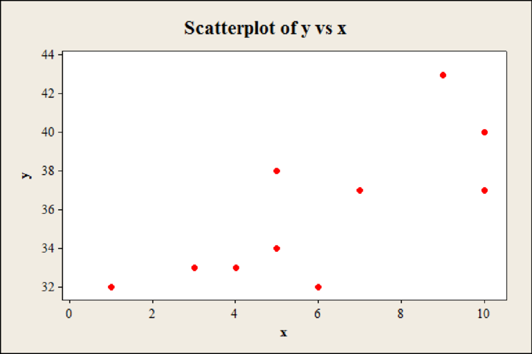
The scatter diagram for data is,
Explanation of Solution
Calculation:
The variable x denotes the number of job changes and y denotes the annual salary for people living in the Nashville area.
Step by step procedure to obtain scatter plot using MINITAB software is given below:
- Choose Graph > Scatterplot.
- Choose Simple. Click OK.
- In Y variables, enter the column of x.
- In X variables, enter the column of y.
- Click OK.
(b)
Find the value of
Find the value of
Find the value of b.
Find the equation of the least-squares line.
Construct the line on the scatter diagram.
(b)
Answer to Problem 6CRP
The value of
The value of
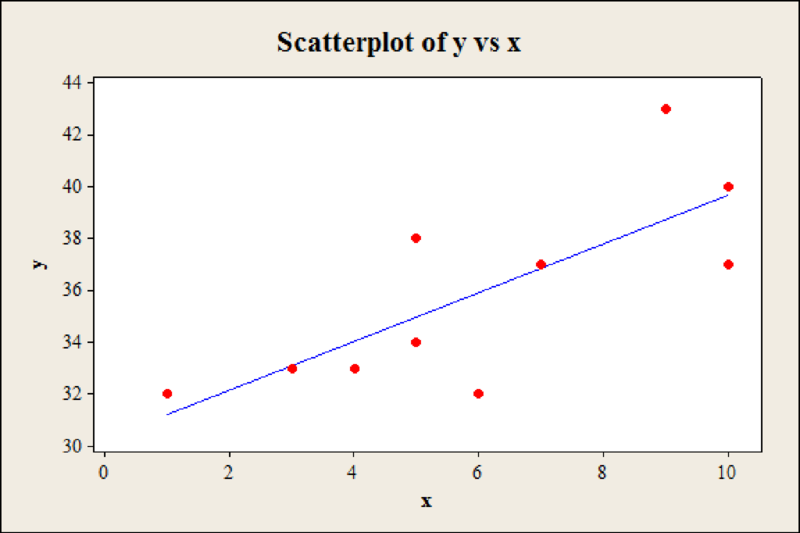
The value of b is 0.939.
The equation of the least-squares line is
The scatter plot the regression line is,
Explanation of Solution
Calculation:
The values are
The value of
Hence, the value of
The value of
Hence, the value of
The value of b is,
Hence, the value of b is 0.939024.
The value of a is,
The value of a is 30.266.
The equation of the least-squares line is,
Hence, the equation of the least-squares line is
Step by step procedure to obtain scatter plot using MINITAB software is given below:
- Choose Graph > Scatterplot.
- Choose With regression. Click OK.
- In Y variables, enter the column of x.
- In X variables, enter the column of y.
- Click OK.
(c)
Find the sample
Find the value of the coefficient of determination
Mention percentage of the variation in y is explained by the least-squares model.
(c)
Answer to Problem 6CRP
The sample correlation coefficient r is 0.761.
The value of the coefficient of determination
The percentage of the variation in y is explained by the least-squares model is 69.7%.
Explanation of Solution
Calculation:
Coefficient of determination
The coefficient of determination
Step by step procedure to obtain correlation using MINITAB software is given below:
- Choose Stat > Basic Statistics > Correlation.
- In Variable, enter the column as x, y.
- Click OK.
Output using MINITAB software is given below:
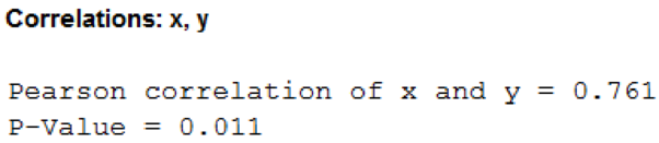
From MINITAB output, the correlation is 0.761.
Hence, the correlation coefficient r is 0.761.
The value of
Hence, the value of the coefficient of determination
About 57.9% of the variation in y (annual salary for people living in the Nashville area) is explained by x (number of job changes). Since the value of
Hence, the percentage of the variation in y that can be explained by variation in x is 57.9%.
(d)
Check whether the claim that the population correlation coefficient is positive or not.
(d)
Answer to Problem 6CRP
The population correlation coefficient is positive.
Explanation of Solution
Calculation:
Null hypothesis:
Alternative hypothesis:
Test statistic:
The test statistic formula for test correlation r is,
Where r is the sample correlation coefficient, n is the sample size with degrees of freedom
Substitute r as 0.761, and n as 10 in the test statistic formula.
The test statistic value is 3.318.
The degrees of freedom is,
Step by step procedure to obtain P-value using MINITAB software is given below:
- Choose Graph > Probability Distribution Plot choose View Probability > OK.
- From Distribution, choose ‘t’ distribution.
- Enter the Degrees of freedom as 8.
- Click the Shaded Area tab.
- Choose X Value and Right Tail, for the region of the curve to shade.
- Enter the X value as 3.318.
- Click OK.
Output using MINITAB software is given below:
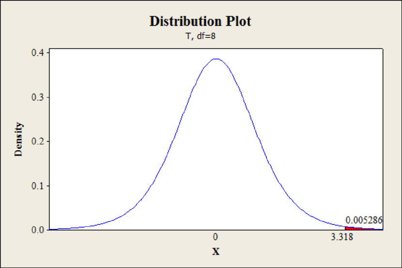
From Minitab output, the P-value is 0.0053.
Rejection rule:
- If the P-value is less than or equal to
Conclusion:
The P-value is 0.0053 and the level of significance is 0.05.
The P-value is less than the level of significance.
That is,
By the rejection rule, the null hypothesis is rejected.
Hence, the population correlation coefficient is positive between the number of job changes and annual salary for people living in the Nashville area.
(e)
Find the least-squares line predicts for y, the annual salary when
(e)
Answer to Problem 6CRP
The least-squares line predicts for y, the annual salary when
Explanation of Solution
Calculation:
From part (b), the equation of the least-squares line is
Substitute
Hence, the least-squares line predicts for y, the annual salary when
(f)
Verify the values of
(f)
Explanation of Solution
Calculation:
The value of
Hence, the value of
(g)
Find the 90% confidence interval for the annual salary of an individual with
(g)
Answer to Problem 6CRP
The 90% confidence interval for the annual salary of an individual with
Explanation of Solution
Calculation:
Step by step procedure to obtain confidence interval using MINITAB software is given below:
- Choose Stat > Regression > Regression.
- In Response, enter the column containing the response as y.
- In Predictors, enter the columns containing the predictor as x.
- Choose Options.
- In Prediction intervals for new observations, enter the value as 2.
- In Confidence level, enter value as 90.
- Click OK.
Output using MINITAB software is given below:
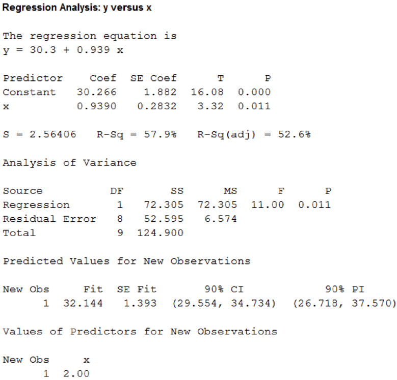
From Minitab output, the confidence interval is
Hence, the 90% confidence interval for the annual salary of an individual with
(h)
Check whether the claim that the slope
(h)
Answer to Problem 6CRP
The slope
Explanation of Solution
Calculation:
Null hypothesis:
Alternative hypothesis:
Test statistic:
From part (g) MINITAB output, the test statistic value is 3.32.
The degrees of freedom is,
Step by step procedure to obtain P-value using MINITAB software is given below:
- Choose Graph > Probability Distribution Plot choose View Probability > OK.
- From Distribution, choose ‘t’ distribution.
- Enter the Degrees of freedom as 8.
- Click the Shaded Area tab.
- Choose X Value and Right Tail, for the region of the curve to shade.
- Enter the X value as 3.32.
- Click OK.
Output using MINITAB software is given below:
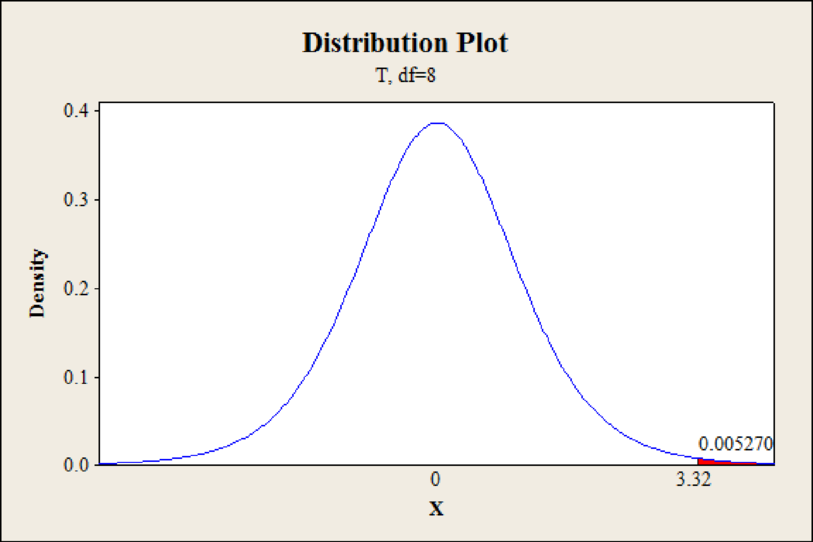
From Minitab output, the P-value is 0.0053.
Conclusion:
The P-value is 0.0053 and the level of significance is 0.05.
The P-value is less than the level of significance.
That is,
By the rejection rule, the null hypothesis is rejected.
Hence, the slope
(i)
Find a 90% confidence interval for
Interpret the confidence interval.
(i)
Answer to Problem 6CRP
The 90% confidence interval for
Explanation of Solution
Calculation:
Confidence interval for slope:
The confidence interval formula for slope
Where
Critical value:
Use the Appendix II: Tables, Table 6: Critical Values for Student’s t Distribution:
- In d.f. column locate the value 8.
- In the row of two-tail area locate the level of significance
- The intersecting value of row and columns is 1.860.
The critical value is
The margin of error is,
The 90% confidence interval for
Hence, the 90% confidence interval for
The annual salary for people living in the Nashville area increases by an amount that ranges between 0.413 and 1.465, if job changes increases by one unit.
Want to see more full solutions like this?
Chapter 9 Solutions
UNDERSTANDABLE STATISTICS(LL)/ACCESS


- Consider the following correlations -0.9 , -0.5 , -0.2 , 0 , 0.2 , 0.5 and 0.9. For each give the fraction of the variation in y that is explained by the least-squares regression of y on x.arrow_forwardSuppose we know the following information about a set of bivariate data: Var(x)=Var(x)=6.95 Cov(x,y)=Cov(x,y)=-2.54 Var(y)=Var(y)=7.45 What is the correlation coefficient of the linear least-squares regression? Round your answer to the nearest hundredth.arrow_forwardIs each of these True or False? (i) The least squares regression line is the line that minimizes the sum of the squares of the residuals. (ii) The least squares regression line must go through as many data points as possible. (iii) If a data point falls on the least squares regression line, then its residual is 0. (iv) The least squares regression line is the line that makes the square of the correlation as small as possible.arrow_forward
- 1. If the number of COVID 19 cases in various states of a country are strongly negatively correlated with the literacy rates, then what should be a likely value of the correlation coefficient? A. 2.11 B. 1.12 C. -5.09 D. -0.92 In problem 1, what should not be a possible line of best fit? A. y = -10 - 7x B. y = 10 - 7x C. y = -5 + 4x D. y = 5 - 4xarrow_forward2. Given the following sets of information, find the linear least squares regression and the correlation coefficient.arrow_forwardA dietitian wishes to see if a person’s cholesterol level will be changed if the diet is supplemented by a certain mineral. Four subjects were pre-tested, and they took the mineral supplement for a 6-week period. The results are shown in the table. Is there sufficient evidence to conclude that the population mean of cholesterol levels has been changed after six weeks at α=0.2α=0.2? Assume that the differences are from an approximately normally distributed population. Subject Cholestrol Level (mg/dl) Cholestrol Level after 6 Weeks (mg/dl) dd ¯dd¯ (d−¯d)2(d-d¯)2 1 206 217 11 2 219 184 -35 3 202 204 2 4 213 205 -8 Total -30 a) Calculate the mean, the sum of the squared deviation from the mean, and the standard deviation of differences. Do not include the unit for each answer: ¯d=d¯= (do not round) ∑(d−¯d)2=∑(d-d¯)2= (do not round) sd=sd= (rounded to one decimal place) b) Perform the hypothesis test in the following steps: Step 1.…arrow_forward
- Suppose that X and Y are unknowns with E(X) = 10, Var (X) = 4, E(Y)=12 and Var (Y) = 100. In addition, suppose that the correlation coefficient of X and Y is .6. Then what is the variance of X-Y?arrow_forwardThe operations manager of a musical instrument distributor feels that the demand for Bass Drums may be related to the number of television appearances by the popular rick group Green Shades during the previous month. The manager has collected the data shown in the following table. Demand for Bass Drums 3 6 7 5 10 8 Green Shades TV appearances 3 4 7 6 8 5 Develop the linear regression equation to forecast. Forecast demand for Bass Drums when Green Shades’ TV appearances are 10. Compute MSE and standard deviation for Problem 8.arrow_forwardEuropean City Change in Hotel Costs U.S. City Change in Hotel Costs Ljubljana -0.009 Birmingham 0.074 Hotel prices worldwide are projected to increase by 3% next year, but is there a difference between Europe and US? Suppose we have projectd changes in hotels cost for 47 randomly selected major European cities and 53 randomly selected major American Cities. Geneva 0.000 Pittsburgh 0.089 Zagreb 0.060 Indianapolis -0.013 Stockholm 0.041 Norfolk 0.070 Tirana 0.082 Boston 0.077 Riga 0.076 Winston-Salem 0.074 Istanbul 0.021 Stockton 0.021 Bucharest 0.073 Laredo 0.024 Budapest 0.045 Corpus Christi 0.088 Part a Minsk 0.023 Portland 0.020 On the basis of the sample results, can we conclude that the mean change in hotels rates in Europe and US are different ? Develop appropriate null and alternative hypotheses. Rome 0.033 St. Paul 0.061 Antwerp 0.012 Memphis 0.086 Reykjavik -0.002 Virginia Beach 0.052 Düsseldorf 0.044…arrow_forward
 MATLAB: An Introduction with ApplicationsStatisticsISBN:9781119256830Author:Amos GilatPublisher:John Wiley & Sons Inc
 Probability and Statistics for Engineering and th...StatisticsISBN:9781305251809Author:Jay L. DevorePublisher:Cengage Learning
 Statistics for The Behavioral Sciences (MindTap C...StatisticsISBN:9781305504912Author:Frederick J Gravetter, Larry B. WallnauPublisher:Cengage Learning
 Elementary Statistics: Picturing the World (7th E...StatisticsISBN:9780134683416Author:Ron Larson, Betsy FarberPublisher:PEARSON
 The Basic Practice of StatisticsStatisticsISBN:9781319042578Author:David S. Moore, William I. Notz, Michael A. FlignerPublisher:W. H. Freeman
 Introduction to the Practice of StatisticsStatisticsISBN:9781319013387Author:David S. Moore, George P. McCabe, Bruce A. CraigPublisher:W. H. Freeman