
Concept explainers
Videos
a.
State the null and alternate hypotheses.
a.
Answer to Problem 22E
The hypotheses are given below:
Null hypothesis:
That is, there is no significant difference between the mean weight loss of two diets (low-carbohydrate diet and low-fat diet).
Alternate hypothesis:
That is, there is a significant difference between the mean weight loss of two diets (low-carbohydrate diet and low-fat diet).
Explanation of Solution
Calculation:
It is given that, the statistics regarding the weight loss of candidates under low-carbohydrate diet is
Hypothesis:
Hypothesis is an assumption about the parameter of the population, and the assumption may or may not be true.
Let
Claim:
Here, the claim is whether the mean weight loss differs between the two diets or not.
The hypotheses are given below:
Null hypothesis:
Null hypothesis is a statement which is tested for statistical significance in the test. The decision criterion indicates whether the null hypothesis will be rejected or not in the favor of alternate hypothesis.
That is, there is no significant difference between the mean weight loss of two diets (low-carbohydrate diet and low-fat diet).
Alternate hypothesis:
Alternate hypothesis is contradictory statement of the null hypothesis
That is, there is a significant difference between the mean weight loss of two diets (low-carbohydrate diet and low-fat diet).
b.
Find the value of t-test statistic.
b.
Answer to Problem 22E
The value of t-test statistic is 1.996454.
Explanation of Solution
Calculation:
Requirements for a small sample t-test:
- The samples must be independent and drawn randomly from the populations.
- Either the sample size must be greater than 30 or the population must be approximately normal.
The test statistic for the small sample t is obtained as follows:
Under the null hypothesis,
Therefore the test statistic is,
Thus, the test statistic is 1.996454.
c.
Find the number of degrees of freedom for the test statistic.
c.
Answer to Problem 22E
The number of degrees of freedom for the test statistic is 76.
Explanation of Solution
Calculation:
Degrees of freedom:
The degrees of freedom for t using computer package is,
The degrees of freedom, when computing by hand is smaller of
The degrees of freedom is,
Thus, the degree of freedom is 76.
d.
Check whether the null hypothesis is rejected at
d.
Answer to Problem 22E
There is not enough evidence to reject the null hypothesis at
There is no significant difference between the mean weight loss of two diets (low-carbohydrate diet and low-fat diet).
Explanation of Solution
P-value:
Step-by-step procedure to obtain the P-value using the MINITAB software:
- Choose Graph > Probability Distribution Plot
- Choose View Probability > OK.
- From Distribution, choose‘t’ distribution.
- In Degrees of freedom, enter 76.
- Click the Shaded Area tab.
- Choose X value and Both Tail for the region of the curve to shade.
- In X-value enter 1.996454.
- Click OK.
Output using the MINITAB software is given below:
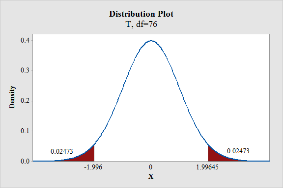
From the MINITAB output, the P-value is
Thus, the P-value is 0.04946.
Decision rule based on P-value:
If
If
Here, the level of significance is
Conclusion based on P-value approach:
The P-value is 0.04946 and
Here, P-value is greater than the
That is,
By the rejection rule, fail to reject the null hypothesis.
Hence, it can be concluded that there is no significant difference between the mean weight loss of two diets (low-carbohydrate diet and low-fat diet).
Thus, it can be concluded that there is sufficient evidence to infer the equality of two population means at
Want to see more full solutions like this?
Chapter 9 Solutions
ESSENTIAL STATISTICS(FD)


 MATLAB: An Introduction with ApplicationsStatisticsISBN:9781119256830Author:Amos GilatPublisher:John Wiley & Sons Inc
 Probability and Statistics for Engineering and th...StatisticsISBN:9781305251809Author:Jay L. DevorePublisher:Cengage Learning
 Statistics for The Behavioral Sciences (MindTap C...StatisticsISBN:9781305504912Author:Frederick J Gravetter, Larry B. WallnauPublisher:Cengage Learning
 Elementary Statistics: Picturing the World (7th E...StatisticsISBN:9780134683416Author:Ron Larson, Betsy FarberPublisher:PEARSON
 The Basic Practice of StatisticsStatisticsISBN:9781319042578Author:David S. Moore, William I. Notz, Michael A. FlignerPublisher:W. H. Freeman
 Introduction to the Practice of StatisticsStatisticsISBN:9781319013387Author:David S. Moore, George P. McCabe, Bruce A. CraigPublisher:W. H. Freeman