
Concept explainers
Videos
(a)
Verify the values of
(a)
Explanation of Solution
Calculation:
The variable x denotes a random variable that represents the percentage of successful free throws a professional basketball player makes in a season and y denotes a random variable that represents the percentage of successful field goals a professional basketball player makes in a season.
The formula for
In the formula, n is the sample size.
The values are verified in the table below,
| x | y | xy | ||
| 67 | 44 | 4489 | 1936 | 2948 |
| 65 | 42 | 4225 | 1764 | 2730 |
| 75 | 48 | 5625 | 2304 | 3600 |
| 86 | 51 | 7396 | 2601 | 4386 |
| 73 | 44 | 5329 | 1936 | 3212 |
| 73 | 51 | 5329 | 2601 | 3723 |
Hence, the values are verified.
The number of data pairs are
Hence, the value of r is verified as approximately 0.784.
(b)
Check whether the claim
(b)
Answer to Problem 7P
The claim
Explanation of Solution
Calculation:
Null hypothesis:
Alternative hypothesis:
Test statistic:
The test statistic formula for test
Where r is the sample correlation coefficient, n is the sample size with degrees of freedom
Substitute r as 0.784, and n as 6 in the test statistic formula.
The test statistic value is 2.526.
The degrees of freedom is,
Step by step procedure to obtain P-value using MINITAB software is given below:
- Choose Graph > Probability Distribution Plot choose View Probability > OK.
- From Distribution, choose ‘t’ distribution.
- Enter the Degrees of freedom as 4.
- Click the Shaded Area tab.
- Choose X Value and Right Tail, for the region of the curve to shade.
- Enter the X value as 2.526.
- Click OK.
Output using MINITAB software is given below:
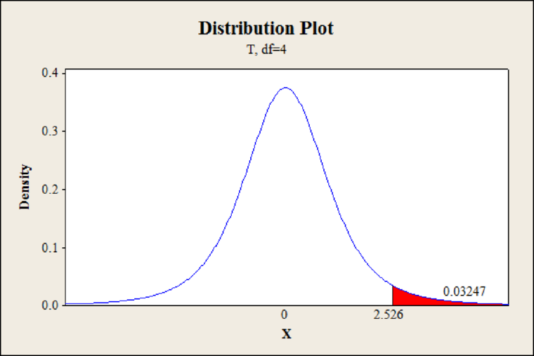
From Minitab output, the P-value is 0.0325.
Rejection rule:
- If the P-value is less than or equal to
Conclusion:
The P-value is 0.0325 and the level of significance is 0.05.
The P-value is less than the level of significance.
That is,
By the rejection rule, the null hypothesis is rejected.
Hence, the claim
(c)
Verify the values of
(c)
Explanation of Solution
Calculation:
The value of
The value of
The value of
The value of
The value of b is,
The value of b is 0.4117.
The value of a is,
The value of a is 16.542.
The value of
The value of
The equation of the least-squares line is,
The regression equation is
(d)
Find the predicted percentage
(d)
Answer to Problem 7P
The predicted percentage
Explanation of Solution
Calculation:
The regression equation is
Substitute x as 70 in the regression equation
Hence, the predicted percentage
(e)
Find the 90% confidence interval for y when
(e)
Answer to Problem 7P
The 90% confidence interval for y when
Explanation of Solution
Calculation:
Step by step procedure to obtain confidence interval using MINITAB software is given below:
- Choose Stat > Regression > Regression.
- In Response, enter the column containing the response as y.
- In Predictors, enter the columns containing the predictor as x.
- Choose Options.
- In Prediction intervals for new observations, enter the value as 70.
- In Confidence level, enter value as 90.
- Click OK.
Output using MINITAB software is given below:
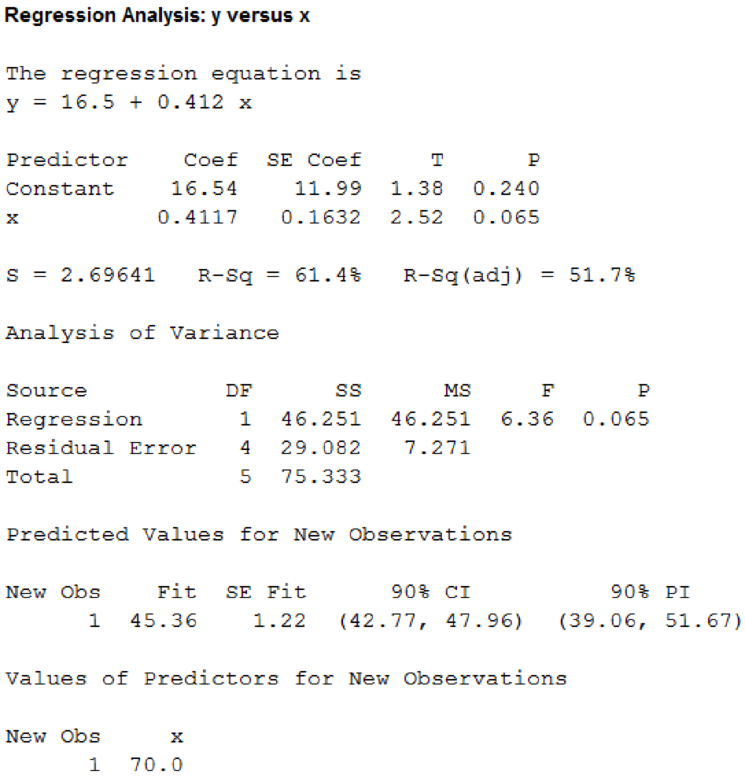
From Minitab output, the confidence interval is
Hence, the 90% confidence interval for y when
(f)
Check whether the claim
(f)
Answer to Problem 7P
The claim
Explanation of Solution
Calculation:
Null hypothesis:
Alternative hypothesis:
Test statistic:
The test statistic formula for slope
Where
Substitute
The test statistic value is 2.522.
The degrees of freedom is,
Step by step procedure to obtain P-value using MINITAB software is given below:
- Choose Graph > Probability Distribution Plot choose View Probability > OK.
- From Distribution, choose ‘t’ distribution.
- Enter the Degrees of freedom as 4.
- Click the Shaded Area tab.
- Choose X Value and Right Tail, for the region of the curve to shade.
- Enter the X value as 2.522.
- Click OK.
Output using MINITAB software is given below:

From Minitab output, the P-value is 0.0326.
Rejection rule:
- If the P-value is less than or equal to
Conclusion:
The P-value is 0.0326 and the level of significance is 0.05.
The P-value is less than the level of significance.
That is,
By the rejection rule, the null hypothesis is rejected.
Hence, the claim
(g)
Find a 90% confidence interval for
Interpret the confidence interval.
(g)
Answer to Problem 7P
The 90% confidence interval for
Explanation of Solution
Calculation:
Confidence interval for slope:
The confidence interval formula for slope
Where
Critical value:
Use the Appendix II: Tables, Table 6: Critical Values for Student’s t Distribution:
- In d.f. column locate the value 4.
- In the row of two-tail area locate the level of significance
- The intersecting value of row and columns is 2.132.
The critical value is
The margin of error is,
The 90% confidence interval for
Hence, the 90% confidence interval for
The percentage of successful field goals for a basketball player increases by an amount that ranges between 0.064 and 0.760, if percentage of successful free throws increases by one unit.
Want to see more full solutions like this?
Chapter 9 Solutions
Bundle: Understandable Statistics: Concepts And Methods, 12th + Webassign, Single-term Printed Access Card


 MATLAB: An Introduction with ApplicationsStatisticsISBN:9781119256830Author:Amos GilatPublisher:John Wiley & Sons Inc
 Probability and Statistics for Engineering and th...StatisticsISBN:9781305251809Author:Jay L. DevorePublisher:Cengage Learning
 Statistics for The Behavioral Sciences (MindTap C...StatisticsISBN:9781305504912Author:Frederick J Gravetter, Larry B. WallnauPublisher:Cengage Learning
 Elementary Statistics: Picturing the World (7th E...StatisticsISBN:9780134683416Author:Ron Larson, Betsy FarberPublisher:PEARSON
 The Basic Practice of StatisticsStatisticsISBN:9781319042578Author:David S. Moore, William I. Notz, Michael A. FlignerPublisher:W. H. Freeman
 Introduction to the Practice of StatisticsStatisticsISBN:9781319013387Author:David S. Moore, George P. McCabe, Bruce A. CraigPublisher:W. H. Freeman