
(a)
The values of gain
Case 1: For
Case 2: For
Case 3: For a root separation factor of 10.
Answer to Problem 10.22P
The values of gains for the PI controller are as follows:
Case 1: For
Case 2: For
Case 3: For a root separation factor of 10,
Explanation of Solution
Given:
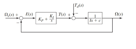
The proportional integral controller of the first order plant is as shown below:
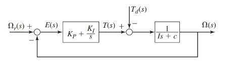
Where, the parameter values are as given:
Also, the performance specifications require the time constant of the system to be
Concept Used:
- The transfer functions for the block diagram are as shown below:
- For a second order system having a characteristic equation of the form
- For a second order system, if the root separation factor is K then, we have following conclusions for the roots and their corresponding time constant, that is
For roots
Also, the corresponding time constant for the system would be
The corresponding time constants of the system would be:
Calculation:
From the block diagram as shown, the transfer functions are as:
Therefore, the characteristic equation for the system is:
On putting the values of parameters in this expression of characteristic equation:
On comparing this equation with form
Undamped natural frequency:
Damping ratio:
Thus, the time constant for the system is:
As the performance specifications require the time constant of the system to be
Therefore, at
Case 1. When
Since,
Case 2. When
Since,
Case 3. When the root separation factor is 10.
For this value of the root separation factor
As given in the question system, performance requires time constant to be 0.2seconds or say the dominant time constant to be 0.2 seconds, then the secondary time constant would be 0.02 seconds. Therefore, the characteristic roots corresponding to these time constants would be:
Thus, the corresponding characteristic equation for the system will be:
On comparing this equation with
And
Conclusion:
The values of gains for the PI controller areas follows:
Case 1. For
Case 2. For
Case 3. For a root separation factor of 10,
(b)
To plot:
The response
Answer to Problem 10.22P
The response
Explanation of Solution
Given:
The proportional integral controller of first order plant is as shown below:
Where, the parameter values are as given:
Also, the performance specifications require the time constant of the system to be
The values of gains for the PI controller are as follows:
Case 1. For
Case 2. For
Case 3. For a root separation factor of 10,
Concept Used:
- The transfer functions for the block diagram are as shown below:
Calculation:
From the block diagram as shown, the transfer functions are as:
Therefore, the response
On putting the values of parameters in this expression of characteristic equation:
Case 1. When
Since,
Therefore, for unit-step command response
On simplifying this response of
On taking inverse Laplace transform of this, we have
Case 2. When
Since,
Therefore, for unit-step command response
On simplifying this response of
On taking inverse Laplace transform of this, we have
Case 3. When the root separation factor is 10.
That is, the gain values are
Since,
Therefore, for unit-step command response
On simplifying this response of
On taking inverse Laplace transform of this, we have
On plotting the responses
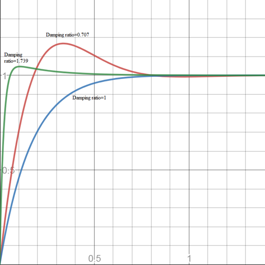
Figure 1
From Figure 1,it is observed that there is a high overshoot in the responseat the damping ratio
Conclusion:
Therefore, the response
Want to see more full solutions like this?
Chapter 10 Solutions
SYSTEM DYNAMICS LL+CONNECT

 Elements Of ElectromagneticsMechanical EngineeringISBN:9780190698614Author:Sadiku, Matthew N. O.Publisher:Oxford University Press
 Mechanics of Materials (10th Edition)Mechanical EngineeringISBN:9780134319650Author:Russell C. HibbelerPublisher:PEARSON
 Thermodynamics: An Engineering ApproachMechanical EngineeringISBN:9781259822674Author:Yunus A. Cengel Dr., Michael A. BolesPublisher:McGraw-Hill Education
 Control Systems EngineeringMechanical EngineeringISBN:9781118170519Author:Norman S. NisePublisher:WILEY
 Mechanics of Materials (MindTap Course List)Mechanical EngineeringISBN:9781337093347Author:Barry J. Goodno, James M. GerePublisher:Cengage Learning
 Engineering Mechanics: StaticsMechanical EngineeringISBN:9781118807330Author:James L. Meriam, L. G. Kraige, J. N. BoltonPublisher:WILEY