
Videos
(a)
To find: The variables IBI and area using numerical method.
(a)
Answer to Problem 48E
Solution: The obtained result can be shown in tabular form as follows:
Variable |
Mean |
Standard deviation |
Area |
28.29 |
17.71 |
IBI |
65.94 |
18.28 |
Explanation of Solution
Calculation: Calculate the average and standard deviation of IBI and area using Minitab as follows:
Step 1: Enter the data in Minitab.
Step 2: Click on Stat --> Basic statistics --> Display
Step 3: Double click on “Area” and “IBI” to move it to variables column.
Step 4: Click on “Statistics” and check the box for mean and standard deviation.
Step 5: Click “OK” twice to obtain the result.
Results are obtained as
Variable |
Mean |
Standard deviation |
Area |
28.29 |
17.71 |
IBI |
65.94 |
18.28 |
To find: The variables IBI and area using graphical method.
Answer to Problem 48E
Solution: The graph of “Area” is slightly right skewed and the graph of “IBI” is left skewed.
Explanation of Solution
Graph: Construct the histograms to check the skewness using Minitab as follows:
Step 1: Go to Graphs > Histogram > Simple histogram.
Step 2: Double click on “Area” and “IBI” to move it to variables column.
Step 3: Click “OK” to obtain the result.
The graph is obtained as
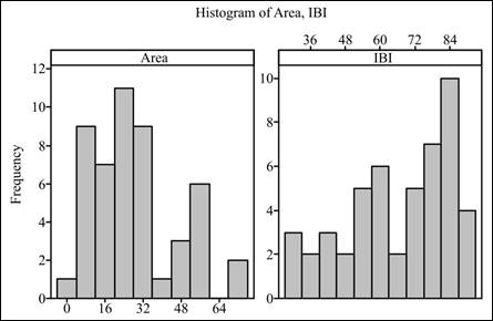
Interpretation: The graph of area is slightly right skewed and the graph of IBI is left skewed.
(b)
To graph: A
(b)
Explanation of Solution
Graph: Construct a scatter plot as follows:
Step 1: Enter the data in Minitab.
Step 2: Click on Graph --> Scatterplot. Select scatterplot with regression.
Step 3: Double click on “IBI” to move it Y variable and “Area” to move it to X variable column.
Step 4: Click “OK” twice to obtain the graph.
The scatter plot is obtained as
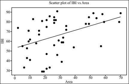
Interpretation: The graph shows weak linear relationship between IBI and Area with no unusual activity.
(c)
To explain: The statistical model for simple linear regression.
(c)
Answer to Problem 48E
Solution: The model is
Explanation of Solution
where
(d)
To explain: The null and alternate hypotheses.
(d)
Answer to Problem 48E
Solution: The null and alternative hypotheses are
Explanation of Solution
So, the null and alternative hypotheses can be stated as
(e)
To test: The least square
(e)
Answer to Problem 48E
Solution: The obtained output represents that the P-value is less than 0.05. So there is enough evidence for the linearity in the regression line.
Explanation of Solution
Calculation: Obtain the regression line using Minitab as follows:
Step 1: Enter the data in Minitab.
Step 2: Click on Stat --> Regression --> Regression.
Step 3: Double click on “IBI” to move it response column and “Area” to move it to predictor column.
Step 4: Click “OK” to obtain the result.
The results are obtained.
Conclusion: From the obtained output, the value of test statistic is 3.42 and the P-value is 0.001. Since the P-value is less than the significance level 0.05, it can be concluded that there is enough evidence for the linearity in the regression line.
(f)
To find: The residuals.
(f)
Answer to Problem 48E
Solution: The residuals are as follows:
Area |
IBI |
Residuals |
21 |
47 |
–15.5862 |
34 |
76 |
7.4318 |
6 |
33 |
–22.6839 |
47 |
78 |
3.4497 |
10 |
62 |
4.4755 |
49 |
78 |
2.5294 |
23 |
33 |
–30.5065 |
32 |
64 |
–3.6479 |
12 |
83 |
24.5552 |
16 |
67 |
6.7146 |
29 |
61 |
–5.2675 |
49 |
85 |
9.5294 |
28 |
46 |
–19.8073 |
8 |
53 |
–3.6042 |
57 |
55 |
–24.1518 |
9 |
71 |
13.9356 |
31 |
59 |
–8.1878 |
10 |
41 |
–16.5245 |
21 |
82 |
19.4138 |
26 |
56 |
–8.8870 |
31 |
39 |
–28.1878 |
52 |
89 |
12.1490 |
21 |
32 |
–30.5862 |
8 |
43 |
–13.6042 |
18 |
29 |
–32.2058 |
5 |
55 |
–0.2237 |
18 |
81 |
19.7942 |
26 |
82 |
17.1130 |
27 |
82 |
16.6529 |
26 |
85 |
20.1130 |
32 |
59 |
–8.6479 |
2 |
74 |
20.1567 |
59 |
80 |
–0.0721 |
58 |
88 |
8.3880 |
19 |
29 |
–32.6659 |
14 |
58 |
–1.3651 |
16 |
71 |
10.7146 |
9 |
60 |
2.9356 |
23 |
86 |
22.4935 |
28 |
91 |
25.1927 |
34 |
72 |
3.4318 |
70 |
89 |
3.8662 |
69 |
80 |
–4.6737 |
54 |
84 |
6.2287 |
39 |
54 |
–16.8690 |
9 |
71 |
13.9356 |
21 |
75 |
12.4138 |
54 |
84 |
6.2287 |
26 |
79 |
14.1130 |
Explanation of Solution
Calculation: Obtain the regression line using Minitab as follows:
Step 1: Enter the data in Minitab.
Step 2: Click on Stat --> Regression --> Regression.
Step 3: Double click on “IBI” to move it to response column and “Area” to move it to predictor column.
Step 4: Click on “Storage” and check the box for residuals.
Step 5: Click “OK” twice to obtain the result.
To graph: The scatterplot.
Explanation of Solution
Graph: Construct a scatterplot using Minitab as follows:
Step 1: Enter the data in Minitab.
Step 2: Click on Graph --> Scatterplot. Select scatterplot with regression.
Step 3: Double click on “Area” to move it X variable and “Residuals” to move it to Y variable column.
Step 4: Click “OK” to obtain the graph.
The scatter plot is obtained as
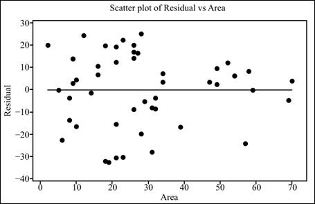
Interpretation: The graph shows that there is more variation for small
Whether there is something unusual.
Answer to Problem 48E
Solution: No, there is nothing unusual.
Explanation of Solution
(g)
That residuals are normal or not.
(g)
Answer to Problem 48E
Solution: The residuals are
Explanation of Solution
Step 1: Click on Stat --> Descriptive statistics --> Normality test.
Step 2: Double click on “Residuals” to move it to the variable column.
Step 3: Click “OK” to obtain the graph.
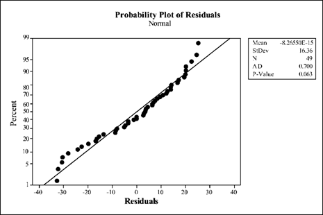
Conclusion: All the points lie near the trend line and there are no outliers. Therefore, it can be concluded that residuals are normally distributed.
(h)
If the assumptions of statistical inference are satisfied or not.
(h)
Answer to Problem 48E
Solution: The assumptions are satisfied.
Explanation of Solution
Want to see more full solutions like this?
Chapter 10 Solutions
Introduction to the Practice of Statistics


 MATLAB: An Introduction with ApplicationsStatisticsISBN:9781119256830Author:Amos GilatPublisher:John Wiley & Sons Inc
 Probability and Statistics for Engineering and th...StatisticsISBN:9781305251809Author:Jay L. DevorePublisher:Cengage Learning
 Statistics for The Behavioral Sciences (MindTap C...StatisticsISBN:9781305504912Author:Frederick J Gravetter, Larry B. WallnauPublisher:Cengage Learning
 Elementary Statistics: Picturing the World (7th E...StatisticsISBN:9780134683416Author:Ron Larson, Betsy FarberPublisher:PEARSON
 The Basic Practice of StatisticsStatisticsISBN:9781319042578Author:David S. Moore, William I. Notz, Michael A. FlignerPublisher:W. H. Freeman
 Introduction to the Practice of StatisticsStatisticsISBN:9781319013387Author:David S. Moore, George P. McCabe, Bruce A. CraigPublisher:W. H. Freeman