
Concept explainers
Videos
(a)
Section 1:
To graph: A
(a)
Section 1:
Explanation of Solution
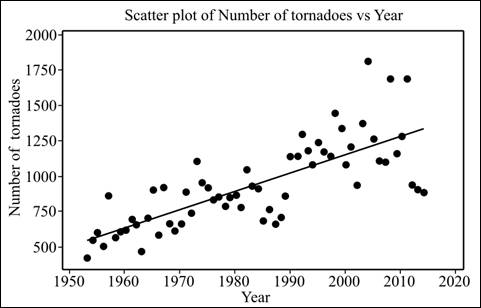
Graph: Construct a scatterplot using Minitab as follows:
Step 1: Enter the data in Minitab.
Step 2: Click on Graph --> Scatterplot. Select scatterplot with regression.
Step 3: Double click on ‘Number of tornadoes’ to move it to Y variable and ‘Year’ to move it to X variable column.
Step 4: Click ‘Ok’ twice to obtain the graph.
Section 2:
To explain: The relationship between two variables seems linear.
Section 2:
Answer to Problem 19E
Solution: The variables are in linear relationship.
Explanation of Solution
Section 3:
To explain: Whether there are any outliers or unusual pattern.
Section 3:
Answer to Problem 19E
Solution: There are no outliers.
Explanation of Solution
(b)
To find: The least square regression line.
(b)
Answer to Problem 19E
Solution: The regression line is:
Explanation of Solution
Calculation: Obtain the regression line using Minitab as follows:
Step 1: Enter the data in Minitab.
Step 2: Click on Stat --> Regression --> Regression.
Step 3: Double click on ‘Number of tornadoes’ to move it to Y variable and ‘Year’ to move it to X variable column.
Step 4: Click on ‘Storage’ and check the box for residuals.
Step 5: Click ‘Ok’ twice to obtain the result.
Hence, the obtained regression line is
(c)
To explain: The intercept of regression equation.
(c)
Answer to Problem 19E
Solution: The fit is correct because intercept is only used when
Explanation of Solution
(d)
Section 1:
To find: The residuals.
(d)
Section 1:
Answer to Problem 19E
Solution: The residuals are as follows:
Years |
Number of tornadoes |
Residuals |
1953 |
421 |
-127.661 |
1954 |
550 |
-11.495 |
1955 |
593 |
18.670 |
1956 |
504 |
-83.164 |
1957 |
856 |
256.001 |
1958 |
564 |
-48.833 |
1959 |
604 |
-21.668 |
1960 |
616 |
-22.502 |
1961 |
697 |
45.663 |
1962 |
657 |
-7.171 |
1963 |
464 |
-213.006 |
1964 |
704 |
14.160 |
1965 |
906 |
203.325 |
1966 |
585 |
-130.509 |
1967 |
926 |
197.656 |
1968 |
660 |
-81.178 |
1969 |
608 |
-146.013 |
1970 |
653 |
-113.847 |
1971 |
888 |
108.318 |
1972 |
741 |
-51.516 |
1973 |
1102 |
296.649 |
1974 |
947 |
128.815 |
1975 |
920 |
88.980 |
1976 |
835 |
-8.854 |
1977 |
852 |
-4.689 |
1978 |
788 |
-81.523 |
1979 |
852 |
-30.358 |
1980 |
866 |
-29.192 |
1981 |
783 |
-125.027 |
1982 |
1046 |
125.139 |
1983 |
931 |
-2.696 |
1984 |
907 |
-39.530 |
1985 |
684 |
-275.365 |
1986 |
764 |
-208.199 |
1987 |
656 |
-329.034 |
1988 |
702 |
-295.868 |
1989 |
856 |
-154.703 |
1990 |
1133 |
109.463 |
1991 |
1132 |
95.628 |
1992 |
1298 |
248.794 |
1993 |
1176 |
113.959 |
1994 |
1082 |
7.125 |
1995 |
1235 |
147.290 |
1996 |
1173 |
72.456 |
1997 |
1148 |
34.621 |
1998 |
1449 |
322.787 |
1999 |
1340 |
200.952 |
2000 |
1075 |
-76.882 |
2001 |
1215 |
50.283 |
2002 |
934 |
-243.551 |
2003 |
1374 |
183.614 |
2004 |
1817 |
613.780 |
2005 |
1265 |
48.945 |
2006 |
1103 |
-125.889 |
2007 |
1096 |
-145.724 |
2008 |
1692 |
437.442 |
2009 |
1156 |
-111.393 |
2010 |
1282 |
1.773 |
2011 |
1691 |
397.938 |
2012 |
938 |
-367.896 |
2013 |
907 |
-411.731 |
2014 |
888 |
-443.565 |
Explanation of Solution
Calculation: Obtain the residuals using Minitab as follows:
Step 1: Enter the data in Minitab.
Step 2: Click on Stat --> Regression --> Regression.
Step 3: Double click on ‘Number of tornadoes’ to move it response column and ‘Year’ to move it to predictor column.
Step 4: Click on ‘Storage’ and check the box for residuals.
Step 5: Click ‘Ok’ to obtain the result.
Hence, the obtained residuals are shown below:
Years |
Number of tornadoes |
Residuals |
1953 |
421 |
-127.661 |
1954 |
550 |
-11.495 |
1955 |
593 |
18.670 |
1956 |
504 |
-83.164 |
1957 |
856 |
256.001 |
1958 |
564 |
-48.833 |
1959 |
604 |
-21.668 |
1960 |
616 |
-22.502 |
1961 |
697 |
45.663 |
1962 |
657 |
-7.171 |
1963 |
464 |
-213.006 |
1964 |
704 |
14.160 |
1965 |
906 |
203.325 |
1966 |
585 |
-130.509 |
1967 |
926 |
197.656 |
1968 |
660 |
-81.178 |
1969 |
608 |
-146.013 |
1970 |
653 |
-113.847 |
1971 |
888 |
108.318 |
1972 |
741 |
-51.516 |
1973 |
1102 |
296.649 |
1974 |
947 |
128.815 |
1975 |
920 |
88.980 |
1976 |
835 |
-8.854 |
1977 |
852 |
-4.689 |
1978 |
788 |
-81.523 |
1979 |
852 |
-30.358 |
1980 |
866 |
-29.192 |
1981 |
783 |
-125.027 |
1982 |
1046 |
125.139 |
1983 |
931 |
-2.696 |
1984 |
907 |
-39.530 |
1985 |
684 |
-275.365 |
1986 |
764 |
-208.199 |
1987 |
656 |
-329.034 |
1988 |
702 |
-295.868 |
1989 |
856 |
-154.703 |
1990 |
1133 |
109.463 |
1991 |
1132 |
95.628 |
1992 |
1298 |
248.794 |
1993 |
1176 |
113.959 |
1994 |
1082 |
7.125 |
1995 |
1235 |
147.290 |
1996 |
1173 |
72.456 |
1997 |
1148 |
34.621 |
1998 |
1449 |
322.787 |
1999 |
1340 |
200.952 |
2000 |
1075 |
-76.882 |
2001 |
1215 |
50.283 |
2002 |
934 |
-243.551 |
2003 |
1374 |
183.614 |
2004 |
1817 |
613.780 |
2005 |
1265 |
48.945 |
2006 |
1103 |
-125.889 |
2007 |
1096 |
-145.724 |
2008 |
1692 |
437.442 |
2009 |
1156 |
-111.393 |
2010 |
1282 |
1.773 |
2011 |
1691 |
397.938 |
2012 |
938 |
-367.896 |
2013 |
907 |
-411.731 |
2014 |
888 |
-443.565 |
Section 2:
To graph: The scatterplot of residual versus year.
Section 2:
Explanation of Solution
Graph: Construct a scatterplot using Minitab as follows:
Step 1: Enter the data in Minitab.
Step 2: Click on Graph --> Scatterplot. Select scatterplot with regression.
Step 3: Double click on ‘Residuals’ to move it to Y variable and ‘Year’ to move it to X variable column.
Step 4: Click ‘Ok’ to obtain the graph.
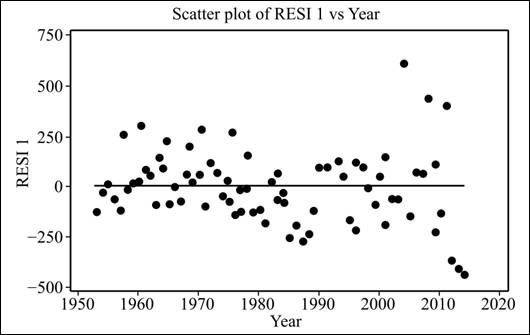
From the scatter plot, it is clear that the residual plot looks mostly random
(e)
To explain: That residuals are normal or not.
(e)
Answer to Problem 19E
Solution: The residuals are
Explanation of Solution
Graph: Construct the probability plot for residuals to test for the normality using Minitab as follows:
Step 1: Click on Stat -->
Step 2: Double click on ‘Residuals’ to move it to the variable column.
Step 3: Click ‘OK’ to obtain the graph.
Hence, the obtained graph is shown below:
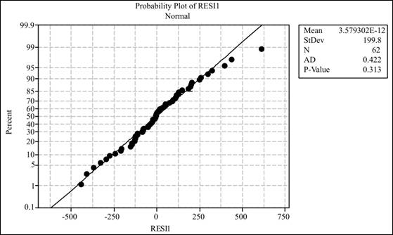
Interpretation: All the points lie near the trend line. Therefore, it can be concluded that residuals are normally distributed.
(f)
To explain: The accuracy of inference based on residual checks.
(f)
Answer to Problem 19E
Solution: The inference can be made based on residuals.
Explanation of Solution
Want to see more full solutions like this?
Chapter 10 Solutions
Introduction to the Practice of Statistics


 MATLAB: An Introduction with ApplicationsStatisticsISBN:9781119256830Author:Amos GilatPublisher:John Wiley & Sons Inc
 Probability and Statistics for Engineering and th...StatisticsISBN:9781305251809Author:Jay L. DevorePublisher:Cengage Learning
 Statistics for The Behavioral Sciences (MindTap C...StatisticsISBN:9781305504912Author:Frederick J Gravetter, Larry B. WallnauPublisher:Cengage Learning
 Elementary Statistics: Picturing the World (7th E...StatisticsISBN:9780134683416Author:Ron Larson, Betsy FarberPublisher:PEARSON
 The Basic Practice of StatisticsStatisticsISBN:9781319042578Author:David S. Moore, William I. Notz, Michael A. FlignerPublisher:W. H. Freeman
 Introduction to the Practice of StatisticsStatisticsISBN:9781319013387Author:David S. Moore, George P. McCabe, Bruce A. CraigPublisher:W. H. Freeman