
Concept explainers
Videos
(a)
To find: The variables IBI and Forest using numerical method.
(a)
Answer to Problem 49E
Solution: The obtained result can be shown in tabular form as follows:
Variable |
Mean |
Standard deviation |
Forest |
39.39 |
32.20 |
IBI |
65.94 |
18.28 |
Explanation of Solution
Calculation: Calculate the average and standard deviation of IBI and Forest using Minitab as follows:
Step 1: Enter the data in Minitab.
Step 2: Go to Graphs > Histogram > Simple histogram.
Step 3: Double click on ‘Forest’ and ‘IBI’ to move it to variables column.
Step 4: Click on ‘Statistics’ and check the box for mean and standard deviation.
Step 5: Click ‘OK’ twice to obtain the result.
Results are obtained as:
Variable |
Mean |
Standard deviation |
Forest |
39.39 |
32.20 |
IBI |
65.94 |
18.28 |
To find: The variables IBI and Forest using graphical method.
Answer to Problem 49E
Solution: The graph of Forest is right skewed and the graph of IBI is left skewed.
Explanation of Solution
Graph: Construct the histograms to check the skewness using Minitab as follows:
Step 1: Click on Graphs --> Histogram. Select simple histogram.
Step 2: Double click on ‘Forest’ and ‘IBI’ to move it to variables column.
Step 3: Click ‘OK’ to obtain the result.
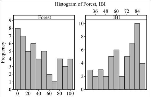
Interpretation: The graph of Forest is right skewed and the graph of IBI is left skewed.
(b)
To graph: A
(b)
Explanation of Solution
Graph: Construct a scatter plot as follows:
Step 1: Enter the data in Minitab.
Step 2: Click on Graph --> Scatterplot. Select scatterplot with regression.
Step 3: Double click on ‘BAC’ to move it Y variable and ‘Beer’ to move it to X variable column.
Step 4: Click ‘Ok’ twice to obtain the graph.
The scatter plot is obtained as:
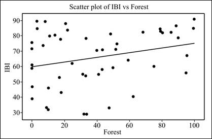
Interpretation: The graph shows weak linear relationship between IBI and Forest with no unusual activity.
(c)
To explain: The statistical model for simple linear regression.
(c)
Answer to Problem 49E
Solution: The model is
Explanation of Solution
Where,
(d)
To explain: The null and alternate hypotheses.
(d)
Answer to Problem 49E
Solution: The null and alternative hypotheses are:
Explanation of Solution
So, the null and alternative hypothesis can be stated as:
(e)
To test: The least square
(e)
Answer to Problem 49E
Solution: The obtained output represents that the p-value is greater than 0.05. So there is no enough evidence for the linearity in the regression line.
Explanation of Solution
Calculation: Obtain the regression line using Minitab as follows:
Step 1: Enter the data in Minitab.
Step 2: Click on Stat --> Regression --> Regression.
Step 3: Double click on ‘IBI’ to move it response column and ‘Forest’ to move it to predictor column.
Step 4: Click ‘Ok’ to obtain the result.
Conclusion: From the obtained output the value of test statistic is 1.92 and the p-value is 0.061. Since the p-value is greater than 0.05, it can be concluded that there is no enough evidence for the linearity in the regression line
(f)
To find: The residuals.
(f)
Answer to Problem 49E
Solution: The residuals are as follows:
Forest |
IBI |
Residuals |
0 |
47 |
-12.9072 |
0 |
76 |
16.0928 |
9 |
33 |
-28.2854 |
17 |
78 |
15.4895 |
25 |
62 |
-1.7355 |
33 |
78 |
13.0394 |
47 |
33 |
-34.1045 |
59 |
64 |
-4.9420 |
79 |
83 |
10.9953 |
95 |
67 |
-7.4548 |
0 |
61 |
1.0928 |
3 |
85 |
24.6334 |
10 |
46 |
-15.4386 |
17 |
53 |
-9.5105 |
31 |
55 |
-9.6543 |
39 |
71 |
5.1206 |
49 |
59 |
-8.4107 |
63 |
41 |
-28.5546 |
80 |
82 |
9.8422 |
95 |
56 |
-18.4548 |
0 |
39 |
-20.9072 |
3 |
89 |
28.6334 |
10 |
32 |
-29.4386 |
18 |
43 |
-19.6636 |
32 |
29 |
-35.8075 |
41 |
55 |
-11.1857 |
49 |
81 |
13.5893 |
68 |
82 |
11.6798 |
86 |
82 |
8.9234 |
100 |
85 |
9.7795 |
0 |
59 |
-0.9072 |
7 |
74 |
13.0208 |
11 |
80 |
18.4083 |
21 |
88 |
24.8770 |
33 |
29 |
-35.9606 |
43 |
58 |
-8.4919 |
52 |
71 |
3.1299 |
75 |
60 |
-11.3922 |
89 |
86 |
12.4640 |
100 |
91 |
15.7795 |
0 |
72 |
12.0928 |
8 |
89 |
27.8677 |
14 |
80 |
17.9489 |
22 |
84 |
20.7238 |
33 |
54 |
-10.9606 |
43 |
71 |
4.5081 |
52 |
75 |
7.1299 |
79 |
84 |
11.9953 |
90 |
79 |
5.3109 |
Explanation of Solution
Calculation: Obtain the regression line using Minitab as follows:
Step 1: Enter the data in Minitab.
Step 2: Click on Stat --> Regression --> Regression.
Step 3: Double click on ‘IBI’ to move it response column and ‘Forest’ to move it to predictor column.
Step 4: Click on ‘Storage’ and check the box for residuals.
Step 5: Click ‘Ok’ twice to obtain the result.
To graph: The scatterplot.
Explanation of Solution
Graph: Construct a scatterplot using Minitab as follows:
Step 1: Enter the data in Minitab.
Step 2: Click on Graph --> Scatterplot. Select scatterplot with regression.
Step 3: Double click on ‘Forest’ to move it X variable and ‘Residuals’ to move it to Y variable column.
Step 4: Click ‘Ok’ to obtain the graph.
The scatter plot is obtained as:
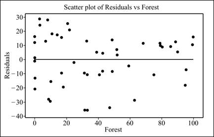
Interpretation: The graph shows that there is more variation for small
To explain: Whether there is something unusual.
Answer to Problem 49E
Solution: No, there is nothing unusual.
Explanation of Solution
(g)
To find: That residuals are normal or not.
(g)
Answer to Problem 49E
Solution: The residuals are approximately
Explanation of Solution
Step 1: Click on Stat -->
Step 2: Double click on ‘Residuals’ to move it to the variable column.
Step 3: Click ‘OK’ to obtain the graph.
The graph is obtained.
Interpretation: All the points lie near the trend line. Therefore, it can be concluded that residuals are approximately normally distributed.
(h)
To explain: If the assumptions of statistical inference in satisfied or not.
(h)
Answer to Problem 49E
Solution: The assumptions are not reasonable.
Explanation of Solution
Want to see more full solutions like this?
Chapter 10 Solutions
Introduction to the Practice of Statistics


 MATLAB: An Introduction with ApplicationsStatisticsISBN:9781119256830Author:Amos GilatPublisher:John Wiley & Sons Inc
 Probability and Statistics for Engineering and th...StatisticsISBN:9781305251809Author:Jay L. DevorePublisher:Cengage Learning
 Statistics for The Behavioral Sciences (MindTap C...StatisticsISBN:9781305504912Author:Frederick J Gravetter, Larry B. WallnauPublisher:Cengage Learning
 Elementary Statistics: Picturing the World (7th E...StatisticsISBN:9780134683416Author:Ron Larson, Betsy FarberPublisher:PEARSON
 The Basic Practice of StatisticsStatisticsISBN:9781319042578Author:David S. Moore, William I. Notz, Michael A. FlignerPublisher:W. H. Freeman
 Introduction to the Practice of StatisticsStatisticsISBN:9781319013387Author:David S. Moore, George P. McCabe, Bruce A. CraigPublisher:W. H. Freeman