
Concept explainers
Videos
Regression and Predictions. Exercises 13–28 use the same data sets as Exercises 13–28 in Section 10-1. In each case, find the regression equation, letting the first variable be the predictor (x) variable, hind the indicated predicted value by following the prediction procedure summarized in Figure 10-5 on page 493.
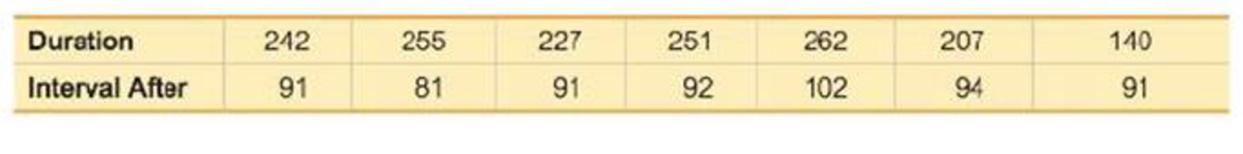
14. Old Faithful Using the listed duration and interval after times, find the best predicted “interval after’’ time for an eruption with a duration of 253 seconds. How does it compare to an actual eruption with a duration of 253 seconds and an interval after time of 83 minutes?

Learn your wayIncludes step-by-step video

Chapter 10 Solutions
MyLab Statistics with Pearson eText -- Standalone Access Card -- for Essentials of Statistics
Additional Math Textbook Solutions
Intro Stats, Books a la Carte Edition (5th Edition)
Elementary Statistics: Picturing the World (6th Edition)
Introductory Statistics (2nd Edition)
Basic Business Statistics, Student Value Edition (13th Edition)
Statistical Reasoning for Everyday Life (5th Edition)


- Using the data in Table 6–11, calculate a 3-month moving average forecast for month 12.arrow_forwardsection 4.1 #30 In Exercises 25–30, determine whether the association between the two variables is positive or negative. Weekly ice cream sales and weekly average temperaturearrow_forwarda.State the predictors available in this model.arrow_forward
- National Debt The size of the total debt owed by the UnitedStates federal government continues to grow. In fact,according to the Department of the Treasury, the debt perperson living in the United States is approximately $53,000(or over $140,000 per U.S. household). The following datarepresent the U.S. debt for the years 2001–2014. Since thedebt D depends on the year y, and each input correspondsto exactly one output, the debt is a function of the year. SoD1y2 represents the debt for each year y. Source: www.treasurydirect.govDebt (billions Debt (billionsYear of dollars) Year of dollars)2001 5807 2008 10,0252002 6228 2009 11,9102003 6783 2010 13,5622004 7379 2011 14,7902005 7933 2012 16,0662006 8507 2013 16,7382007 9008 2014 17,824 (a) Plot the points 12001, 58072, 12002, 62282, and so on ina Cartesian plane.(b) Draw a line segment from the point 12001, 58072 to12006, 85072. What does the slope of this line segmentrepresent?(c) Find the average rate of change of the debt from 2002…arrow_forward(a) For United States, provide data for the variables below over the years 1993 –2007:(i) Net migration rate (per 1,000 population)(ii) Total fertility rate (live births per woman)(iii)Unemployment, general level (Thousands)(iv) Wages(v) Life expectancy at birth for both sexes combined (years)Data can be obtained from the UN database http://data.un.org/Explorer.aspxUsing R-Studio, estimate a regression equation to determine the effect of unemployment,general level, wages and life expectancy at birth for both sexes on the net migration rate.(All codes and regression output should be provided).(i) Write down the regression equation. (ii) Interpret the coefficients and determine which of the individual coefficients in theregression model are statistically significant. In responding, construct and test anyappropriate hypothesis. (iii) Interpret the coefficient of determination.arrow_forward(a) For United States, provide data for the variables below over the years 1993 – 2007: (i) Net migration rate (per 1,000 population) (ii) Total fertility rate (live births per woman) (iii)Unemployment, general level (Thousands) (iv) Wages (v) Life expectancy at birth for both sexes combined (years) Data can be obtained from the UN database http://data.un.org/Explorer.aspx Using R-Studio, estimate a regression equation to determine the effect of unemployment, general level, wages and life expectancy at birth for both sexes on the net migration rate. (All codes and regression output should be provided).(b) Using R-Studio redo the regression analysis with the total fertility rate as an additionalindependent variable. (All codes and regression output should be provided).(i) Write down the regression equation. (ii) Use the 5% level of significance, determine and discuss whether the total fertilityrate has a significant impact on the net migration rate in your assigned country.…arrow_forward
- Heart rate during laughter. Laughter is often called “the best medicine,” since studies have shown that laughter can reduce muscle tension and increase oxygenation of the blood. In the International Journal of Obesity (Jan. 2007), researchers at Vanderbilt University investigated the physiological changes that accompany laughter. Ninety subjects (18–34 years old) watched film clips designed to evoke laughter. During the laughing period, the researchers measured the heart rate (beats per minute) of each subject, with the following summary results: Mean = 73.5, Standard Deviation = 6. n=90 (we can treat this as a large sample and use z) It is well known that the mean resting heart rate of adults is 71 beats per minute. Based on the research on laughter and heart rate, we would expect subjects to have a higher heart beat rate while laughing.Construct 95% Confidence interval using z value. What is the lower bound of CI? a) Calculate the value of the test statistic.(z*) b) If…arrow_forward(a) For United States, provide data for the variables below over the years 1993 – 2007: (i) Net migration rate (per 1,000 population) (ii) Total fertility rate (live births per woman) (iii)Unemployment, general level (Thousands) (iv) Wages (v) Life expectancy at birth for both sexes combined (years) Data can be obtained from the UN database http://data.un.org/Explorer.aspx Using R-Studio, estimate a regression equation to determine the effect of unemployment, general level, wages and life expectancy at birth for both sexes on the net migration rate. (All codes and regression output should be provided). (iv) Using the 10% level of significance, determine and discuss whether the overall regression equation is statistically significant. In responding, construct and test any appropriate hypothesis. (v) Determine and interpret the confidence interval for the independent variable(s).arrow_forward10 – 11. Margaret, an archeologist, is conducting a test to determine if there is a positive linear relationship between the total height of a dinosaur and its leg length. Her random sample of 15 dinosaur total heights (in feet) and leg lengths (in feet) produced the results shown in the following TI calculator screen. Use the TI calculations in the screen shot to help you answer questions: 10 & 11. LinReg y=a+bx a=28.67845743 b=5.639892354 r=559696513 r=.7481286741 10. What would you predict for a dinosaur's total height (to 2 decimal places) in feet, if the leg length is 5.8 feet? a) 61.39 feet b) 28.68 feet c) 114.99 feet d) 61.33 feet e) 74.81 feet 11. What percent of variation in the dinosaur's total height can be accounted for by the variation in the dinosaur's leg length? a) 28.68% b) 5.64%% c) 55.97% d) 74.81% e) none of thesearrow_forward
- In Exercises 13–24, draw a dependency diagram and write a Chain Rule formula for each derivative.arrow_forwardQ1. The table provided gives data on indexes of output per hour (X) and real compensation per hour (Y) for the business and nonfarm business sectors of the U.S. economy for 1960–2005. The base year of the indexes is 1992 = 100 and the indexes are seasonally adjusted. a. Plot Y against X for the two sectors separately. b. What is the economic theory behind the relationship between the two variables? Does the scattergram support the theory? c. Estimate the OLS regression of Y on X. Note: on the table ( 1. Output refers to real gross domestic product in the sector. 2. Wages and salaries of employees plus employers’ contributions for social insurance and private benefit plans. 3. Hourly compensation divided by the consumer price index for all urban consumers for recent quarters.) Thank you!arrow_forwardLarge companies typically collect volumes of data before designing a product, not only to gain information as to whether the product should be released, but also to pinpoint which markets would be the best targets for the product. Several months ago, I was interviewed by such a company while shopping at a mall. I was asked about my exercise habits and whether or not I'd be interested in buying a video/DVD designed to teach stretching exercises. I fall into the male, 18 – 35-years-old category, and I guessed that, like me, many males in that category would not be interested in a stretching video. My friend Amanda falls in the female, older-than-35 category, and I was thinking that she might like the stretching video. After being interviewed, I looked at the interviewer's results. Of the 97 people in my market category who had been interviewed, 16 said they would buy the product, and of the 101 people in Amanda's market category, 31 said they would buy it. Assuming that these data came…arrow_forward
 MATLAB: An Introduction with ApplicationsStatisticsISBN:9781119256830Author:Amos GilatPublisher:John Wiley & Sons Inc
 Probability and Statistics for Engineering and th...StatisticsISBN:9781305251809Author:Jay L. DevorePublisher:Cengage Learning
 Statistics for The Behavioral Sciences (MindTap C...StatisticsISBN:9781305504912Author:Frederick J Gravetter, Larry B. WallnauPublisher:Cengage Learning
 Elementary Statistics: Picturing the World (7th E...StatisticsISBN:9780134683416Author:Ron Larson, Betsy FarberPublisher:PEARSON
 The Basic Practice of StatisticsStatisticsISBN:9781319042578Author:David S. Moore, William I. Notz, Michael A. FlignerPublisher:W. H. Freeman
 Introduction to the Practice of StatisticsStatisticsISBN:9781319013387Author:David S. Moore, George P. McCabe, Bruce A. CraigPublisher:W. H. Freeman