
Concept explainers
Videos
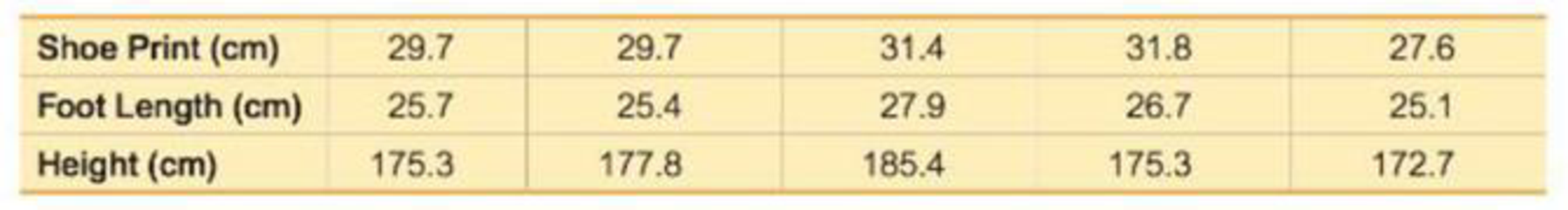
Regression and Predictions. Exercises 13–28 use the same data sets as Exercises 13–28 in Section 10-1. In each case, find the regression equation, letting the first variable be the predictor (x) variable, Find the indicated predicted value by following the prediction procedure summarized in Figure 10-5 on page 493.
17. CSI Statistics Use the shoe print lengths and heights to find the best predicted height of a male who has a shoe print length of 31.3 cm. Would the result be helpful to police crime scene investigators in trying to describe the male?
Want to see the full answer?
Check out a sample textbook solution
Chapter 10 Solutions
MyLab Statistics with Pearson eText -- Standalone Access Card -- for Essentials of Statistics
Additional Math Textbook Solutions
Probability and Statistics for Engineering and the Sciences
Introductory Statistics
Fundamentals of Statistics (5th Edition)
Elementary Statistics
Elementary Statistics Using Excel (6th Edition)
STATISTICS F/BUSINESS+ECONOMICS-TEXT


- section 4.1 #30 In Exercises 25–30, determine whether the association between the two variables is positive or negative. Weekly ice cream sales and weekly average temperaturearrow_forwardUsing the data in Table 6–11, calculate a 3-month moving average forecast for month 12.arrow_forwardUsing the data in Table 6–11, calculate a 3-month moving average forecastfor month 12.arrow_forward
- a.State the predictors available in this model.arrow_forwardMaking Predictions. In Exercises 5–8, let the predictor variable x be the first variable given. Use the given data to find the regression equation and the best predicted value of the response variable. Be sure to follow the prediction procedure summarized in Figure 10-5 on page 493. Use a 0.05 significance level. Bear Measurements Head widths (in.) and weights (lb) were measured for 20 randomly selected bears (from Data Set 9 “Bear Measurements” in Appendix B). The 20 pairs of measurements yield x = 6.9 in., ȳ = 214.3 lb, r = 0.879, P -value = 0.000, and ŷ = −212 + 61.9x. Find the best predicted value of ŷ (weight) given a bear with a head width of 6.5 in.arrow_forwardHeart rate during laughter. Laughter is often called “the best medicine,” since studies have shown that laughter can reduce muscle tension and increase oxygenation of the blood. In the International Journal of Obesity (Jan. 2007), researchers at Vanderbilt University investigated the physiological changes that accompany laughter. Ninety subjects (18–34 years old) watched film clips designed to evoke laughter. During the laughing period, the researchers measured the heart rate (beats per minute) of each subject, with the following summary results: Mean = 73.5, Standard Deviation = 6. n=90 (we can treat this as a large sample and use z) It is well known that the mean resting heart rate of adults is 71 beats per minute. Based on the research on laughter and heart rate, we would expect subjects to have a higher heart beat rate while laughing.Construct 95% Confidence interval using z value. What is the lower bound of CI? a) Calculate the value of the test statistic.(z*) b) If…arrow_forward
- City Fuel Consumption: Finding the Best Multiple Regression Equation. In Exercises 9–12, refer to the accompanying table, which was obtained using the data from 21 cars listed in Data Set 20 “Car Measurements” in Appendix B. The response (y) variable is CITY (fuel consumption in mi/gal). The predictor (x) variables are WT (weight in pounds), DISP (engine displacement in liters), and HWY (highway fuel consumption in mi /gal). If exactly two predictor (x) variables are to be used to predict the city fuel consumption, which two variables should be chosen? Why?arrow_forwardCity Fuel Consumption: Finding the Best Multiple Regression Equation. In Exercises 9–12, refer to the accompanying table, which was obtained using the data from 21 cars listed in Data Set 20 “Car Measurements” in Appendix B. The response (y) variable is CITY (fuel consumption in mi/gal). The predictor (x) variables are WT (weight in pounds), DISP (engine displacement in liters), and HWY (highway fuel consumption in mi /gal). A Honda Civic weighs 2740 lb, it has an engine displacement of 1.8 L, and its highway fuel consumption is 36 mi/gal. What is the best predicted value of the city fuel consumption? Is that predicted value likely to be a good estimate? Is that predicted value likely to be very accurate?arrow_forwardCity Fuel Consumption: Finding the Best Multiple Regression Equation. In Exercises 9–12, refer to the accompanying table, which was obtained using the data from 21 cars listed in Data Set 20 “Car Measurements” in Appendix B. The response (y) variable is CITY (fuel consumption in mi/gal). The predictor (x) variables are WT (weight in pounds), DISP (engine displacement in liters), and HWY (highway fuel consumption in mi /gal). Which regression equation is best for predicting city fuel consumption? Why?arrow_forward
- Large companies typically collect volumes of data before designing a product, not only to gain information as to whether the product should be released, but also to pinpoint which markets would be the best targets for the product. Several months ago, I was interviewed by such a company while shopping at a mall. I was asked about my exercise habits and whether or not I'd be interested in buying a video/DVD designed to teach stretching exercises. I fall into the male, 18 – 35-years-old category, and I guessed that, like me, many males in that category would not be interested in a stretching video. My friend Amanda falls in the female, older-than-35 category, and I was thinking that she might like the stretching video. After being interviewed, I looked at the interviewer's results. Of the 97 people in my market category who had been interviewed, 16 said they would buy the product, and of the 101 people in Amanda's market category, 31 said they would buy it. Assuming that these data came…arrow_forwardNational Debt The size of the total debt owed by the UnitedStates federal government continues to grow. In fact,according to the Department of the Treasury, the debt perperson living in the United States is approximately $53,000(or over $140,000 per U.S. household). The following datarepresent the U.S. debt for the years 2001–2014. Since thedebt D depends on the year y, and each input correspondsto exactly one output, the debt is a function of the year. SoD1y2 represents the debt for each year y. Source: www.treasurydirect.govDebt (billions Debt (billionsYear of dollars) Year of dollars)2001 5807 2008 10,0252002 6228 2009 11,9102003 6783 2010 13,5622004 7379 2011 14,7902005 7933 2012 16,0662006 8507 2013 16,7382007 9008 2014 17,824 (a) Plot the points 12001, 58072, 12002, 62282, and so on ina Cartesian plane.(b) Draw a line segment from the point 12001, 58072 to12006, 85072. What does the slope of this line segmentrepresent?(c) Find the average rate of change of the debt from 2002…arrow_forwardLarge companies typically collect volumes of data before designing a product, not only to gain information as to whether the product should be released, but also to pinpoint which markets would be the best targets for the product. Several months ago, I was interviewed by such a company while shopping at a mall. I was asked about my exercise habits and whether or not I'd be interested in buying a video/DVD designed to teach stretching exercises. I fall into the male, 18 – 35-years-old category, and I guessed that, like me, many males in that category would not be interested in a stretching video. My friend Diane falls in the female, older-than-35 category, and I was thinking that she might like the stretching video. After being interviewed, I looked at the interviewer's results. Of the 93 people in my market category who had been interviewed, 17 said they would buy the product, and of the 113 people in Diane's market category, 34 said they would buy it. Assuming that these data came…arrow_forward
 MATLAB: An Introduction with ApplicationsStatisticsISBN:9781119256830Author:Amos GilatPublisher:John Wiley & Sons Inc
 Probability and Statistics for Engineering and th...StatisticsISBN:9781305251809Author:Jay L. DevorePublisher:Cengage Learning
 Statistics for The Behavioral Sciences (MindTap C...StatisticsISBN:9781305504912Author:Frederick J Gravetter, Larry B. WallnauPublisher:Cengage Learning
 Elementary Statistics: Picturing the World (7th E...StatisticsISBN:9780134683416Author:Ron Larson, Betsy FarberPublisher:PEARSON
 The Basic Practice of StatisticsStatisticsISBN:9781319042578Author:David S. Moore, William I. Notz, Michael A. FlignerPublisher:W. H. Freeman
 Introduction to the Practice of StatisticsStatisticsISBN:9781319013387Author:David S. Moore, George P. McCabe, Bruce A. CraigPublisher:W. H. Freeman