Concept explainers
Videos
Repair and replacement costs of water pipes. Refer to the IHS Journal of Hydraulic Engineering (September 2012) study of water pipes, Exercise 11.12 (p. 622). Recall that a team of civil engineers used
| Diameter (mm) | Ratio | |
| 80 | 6.58 | |
| 100 | 6.97 | |
| 125 | 7.39 | |
| 150 | 7.61 | |
| 200 | 7.78 | |
| 250 | 7.92 | |
| 300 | 8.20 | |
| 350 | 8.42 | |
| 400 | 8.60 | |
| 450 | 8.97 | |
| 500 | 9.31 | |
| 600 | 9.47 | |
| 700 | 9.72 | |
| Source.· eased on ISH Journal or Hydraulic Engineering, Volume 18, Issue 3, pp 241-251. Copyright September 2012 | ||
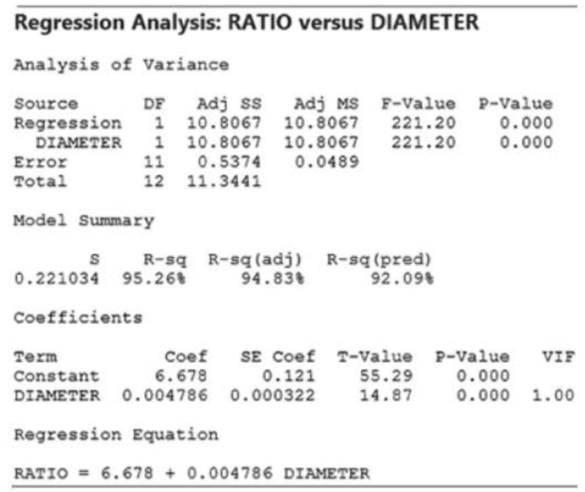
a. Find the least squares line relating ratio of repair to replacement cost (y) to pipe diameter (x) on the printout.
b. Locate the value of SSE on the printout. Is there another line with an average error of 0 that has a smaller SSE than the line, part a? Explain.
c. Interpret, practically, the values
d. Use the regression line to predict the ratio of repair to replacement cost of pipe with a diameter of 800 millimeters.
e. Comment on the reliabilrty of the prediction, part d.
Minitab Output for Exercise 11 .21
Want to see the full answer?
Check out a sample textbook solution
Chapter 11 Solutions
Statistics for Business and Economics (13th Edition)


- A study is conducted to determine if there is a relationship between the two variables, blood haemoglobin (Hb) levels and packed cell volumes (PCV) in the female population. A simple linear regression analysis was performed using SPSS. Based on the SPSS output of the ANOVA table, which of the following statements is the CORRECT interpretation? 1. The regression model statistically significantly predicts the blood haemoglobin level. 2. About 39.98 % of variance in Hb is explained by PCV. 3. The regression model does not fit the data. 4. There is significant contribution of Hb towards PCV.arrow_forwardMr. James, president of Daniel-James Financial Services, believes that there is a relationship between the number of client contacts and the dollar amount of sales. To document this assertion, he gathered the following information from a sample of clients for the last month. Let X represent the number of times that the client was contacted and Y represent the valye of sales ($1000) for each client sampled. Number of Contacts (X) Sales ($1000) 14 24 12 14 20 28 16 30 23 30 a) Compute the regression equation for client contacts and sales. Interpret the slope and intercept parameters.arrow_forwardThe regional transit authority for a major metropolitan area wants to determine whether there is any relationship between the age of a bus and the annual maintenance cost. A sample of 10 buses resulted in the data in Worksheet 2. Worksheet 2 Age of a Bus (years) Maintenance Cost ($) 1 350 2 370 2 480 2 520 2 590 3 550 4 750 4 800 5 790 5 950 Develop a scatter diagram with the age of a bus as the independent variable. Develop the estimated regression equation that can be used to predict the maintenance cost given the age of a bus. Determine the coefficient of determination, and interpret its meaning in this problem. At the 0.05 level of significance, is there evidence of a linear relationship between the age of a bus and the annual maintenance cost.arrow_forward
- For a linear regression for a sample of n=20 pairs of X and Y values. What is the value of the degrees of freedom for the predicted portion of the Y-score variance, MSregression?arrow_forward. A professor at the University of Alabama was interested in evaluating the relationship between family support and delinquency. Using data collected on 4545 families, the researcher used regression to analyze the relationship. The results are presented below. Variables Entered/Removeda Model Variables Entered Variables Removed Method 1 Family supportb . Enter a. Dependent Variable: Delinquency b. All requested variables entered. Model Summary Model R R Square Adjusted R Square Std. Error of the Estimate 1 .249a .062 .062 1.59168 a. Predictors: (Constant), Family support ANOVAa Model Sum of Squares df Mean Square F Sig. 1 Regression 759.204 1 759.204 299.671 <.001b Residual 11479.107 4531 2.533 Total 12238.311 4532 a. Dependent Variable: Delinquency b. Predictors: (Constant), Family support…arrow_forwardA professor at the University of Alabama was interested in evaluating the relationship between family support and delinquency. Using data collected on 4545 families, the researcher used regression to analyze the relationship. The results are presented below. Variables Entered/Removeda Model Variables Entered Variables Removed Method 1 Family supportb . Enter a. Dependent Variable: Delinquency b. All requested variables entered. Model Summary Model R R Square Adjusted R Square Std. Error of the Estimate 1 .249a .062 .062 1.59168 a. Predictors: (Constant), Family support ANOVAa Model Sum of Squares df Mean Square F Sig. 1 Regression 759.204 1 759.204 299.671 <.001b Residual 11479.107 4531 2.533 Total 12238.311 4532 a. Dependent Variable: Delinquency b. Predictors: (Constant), Family support…arrow_forward
- . A professor at the University of Alabama was interested in evaluating the relationship between family support and delinquency. Using data collected on 4545 families, the researcher used regression to analyze the relationship. The results are presented below. Variables Entered/Removeda Model Variables Entered Variables Removed Method 1 Family supportb . Enter a. Dependent Variable: Delinquency b. All requested variables entered. Model Summary Model R R Square Adjusted R Square Std. Error of the Estimate 1 .249a .062 .062 1.59168 a. Predictors: (Constant), Family support ANOVAa Model Sum of Squares df Mean Square F Sig. 1 Regression 759.204 1 759.204 299.671 <.001b Residual 11479.107 4531 2.533 Total 12238.311 4532 a. Dependent Variable: Delinquency b. Predictors: (Constant), Family support…arrow_forwardA professor at the University of Alabama was interested in evaluating the relationship between family support and delinquency. Using data collected on 4545 families, the researcher used regression to analyze the relationship. The results are presented below. Variables Entered/Removeda Model Variables Entered Variables Removed Method 1 Family supportb . Enter a. Dependent Variable: Delinquency b. All requested variables entered. Model Summary Model R R Square Adjusted R Square Std. Error of the Estimate 1 .249a .062 .062 1.59168 a. Predictors: (Constant), Family support ANOVAa Model Sum of Squares df Mean Square F Sig. 1 Regression 759.204 1 759.204 299.671 <.001b Residual 11479.107 4531 2.533 Total 12238.311 4532 a. Dependent Variable: Delinquency b. Predictors: (Constant), Family support…arrow_forwardA professor at the University of Alabama was interested in evaluating the relationship between family support and delinquency. Using data collected on 4545 families, the researcher used regression to analyze the relationship. The results are presented below. Variables Entered/Removeda Model Variables Entered Variables Removed Method 1 Family supportb . Enter a. Dependent Variable: Delinquency b. All requested variables entered. Model Summary Model R R Square Adjusted R Square Std. Error of the Estimate 1 .249a .062 .062 1.59168 a. Predictors: (Constant), Family support ANOVAa Model Sum of Squares df Mean Square F Sig. 1 Regression 759.204 1 759.204 299.671 <.001b Residual 11479.107 4531 2.533 Total 12238.311 4532 a. Dependent Variable: Delinquency b. Predictors: (Constant), Family support…arrow_forward
- The Wall Street Journal asked Concur Technologies, Inc., an expense management company, to examine data from 8.3 million expense reports to provide insights regarding business travel expenses. Their analysis of the data showed that New York was the most expensive city. The following table shows the average daily hotel room rate (X) and the average amount spent on entertainment (Y) for a random sample of 9 of the 25 most-visited U.S. cities. These data lead to the estimated regression equation y = 17.49 + 1.0334x. For these data SSE = 1541.4. Use Table 1 of Appendix B. a. Predict the amount spent on entertainment for a particular city that has a daily room rate of $89 (to 2 decimals). b. Develop a 95% confidence interval for the mean amount spent on entertainment for all cities that have a daily room rate of $89 (to 2 decimals). c. The average room rate in Chicago is $128. Develop a 95% prediction interval for the amount spent on entertainment in Chicago (to 2 decimals).arrow_forwardThe Wall Street Journal asked Concur Technologies, Inc., an expense management company, to examine data from 8.3 million expense reports to provide insights regarding business travel expenses. Their analysis of the data showed that New York was the most expensive city. The following table shows the average daily hotel room rate (X) and the average amount spent on entertainment (Y) for a random sample of 9 of the 25 most-visited U.S. cities. These data lead to the estimated regression equation y = 17.49 + 1.0334x. For these data SSE = 1541.4. Use Table 1 of Appendix B. (NEED ANSWER FOR A) a. Predict the amount spent on entertainment for a particular city that has a daily room rate of $89 (to 2 decimals).arrow_forwardThe owner of Maumee Ford-Mercury-Volvo wants to study the relationship between the age of a car and its selling price. Listed below is a random sample of 12 used cars sold at the dealership during the last year. Car Age Price 1 10 10.8 2 6 9.1 3 12 4.3 4 16 5 5 8 5.1 6 7 11.5 7 9 11.6 8 13 8 9 12 8 10 16 3.9 11 4 12.8 12 4 11.1 Determine the regression equation. (Negative value should be indicated by a minus sign. Round your answers to 3 decimal places.) a= b= Estimate the selling price of a 9-year-old car (in $000). (Round your answer to 3 decimal places.) So for each additional year, the car price decreases ____ in value. Interpret the regression equation (in dollars). (Round your answer to the nearest dollar amount.)arrow_forward
 Glencoe Algebra 1, Student Edition, 9780079039897...AlgebraISBN:9780079039897Author:CarterPublisher:McGraw Hill