
Concept explainers
Videos
a. Consider the data in Exercise 20. Suppose that instead of the least squares line passing through the points (x1, y1),…, (xn, yn) we wish the least squares line passing through
b. Suppose that instead of the model Yi = β0 + β1xi + ϵi (i = 1,…, n), we wish to fit a model of the form
a.
Draw the scatterplot of the points
Draw the scatterplot of the points
Explain the relationship between the least squares lines using the scatterplot.
Answer to Problem 28E
Scatter plot of
Output using MINITAB software is given below:
Scatter plot of
Output using MINITAB software is given below:
The slope of both the plots remains same.
Explanation of Solution
Given info:
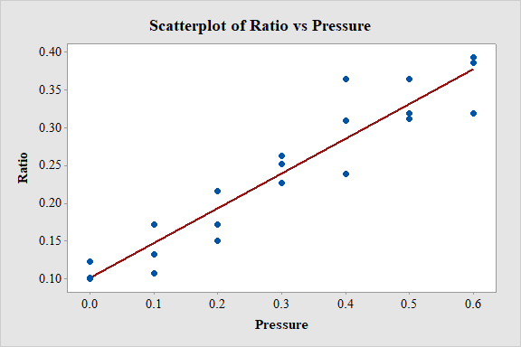
The data represents the values of lateral pressure and the ratio of bond strength expressed in
Justification:
Scatter plot of
Software Procedure:
Step by step procedure to obtain scatterplot using Minitab software is given as,
- Choose Graph > Scatter plot.
- Choose With regression, and then click OK.
- Under Y variables, enter a column of Ratio.
- Under X variables, enter a column of Pressure.
- Click Ok.
Observation:
From the scatterplot it is observed that, as the values of pressure increases the ratio also increases linearly. Thus, there is a positive association between the variables pressure and ratio.
Mean of the variable pressure:
The general formula to obtain mean is,
The points
| i | Ratio | Pressure | |
| 1 | 0.123 | 0 | -6.3 |
| 2 | 0.1 | 0 | -6.3 |
| 3 | 0.101 | 0 | -6.3 |
| 4 | 0.172 | 0.1 | -6.2 |
| 5 | 0.133 | 0.1 | -6.2 |
| 6 | 0.107 | 0.1 | -6.2 |
| 7 | 0.217 | 0.2 | -6.1 |
| 8 | 0.172 | 0.2 | -6.1 |
| 9 | 0.151 | 0.2 | -6.1 |
| 10 | 0.263 | 0.3 | -6 |
| 11 | 0.227 | 0.3 | -6 |
| 12 | 0.252 | 0.3 | -6 |
| 13 | 0.31 | 0.4 | -5.9 |
| 14 | 0.365 | 0.4 | -5.9 |
| 15 | 0.239 | 0.4 | -5.9 |
| 16 | 0.365 | 0.5 | -5.8 |
| 17 | 0.319 | 0.5 | -5.8 |
| 18 | 0.312 | 0.5 | -5.8 |
| 19 | 0.394 | 0.6 | -5.7 |
| 20 | 0.386 | 0.6 | -5.7 |
| 21 | 0.32 | 0.6 | -5.7 |
| Total |
The mean of pressure is,
Thus, the mean of pressure is
Scatter plot of
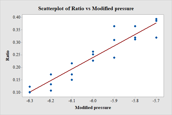
Software Procedure:
Step by step procedure to obtain scatterplot using Minitab software is given as,
- Choose Graph > Scatter plot.
- Choose With regression, and then click OK.
- Under Y variables, enter a column of Ratio.
- Under X variables, enter a column of Modified pressure.
- Click Ok.
Observation:
From the scatterplot it is observed that, as the values of pressure increases the ratio also increases linearly. Thus, there is a positive association between the variables pressure and ratio.
Relationship between the two plots:
The slope of both the plots is same. By subtracting mean from the predictor variable the plot just shifts horizontally without affecting the characteristics.
The least squares line of the points
The least squares line of the points
b.
Derive the least squares estimators of
Explain the relationship between the least squares estimates of the regression line
Answer to Problem 28E
The least squares estimate of slope coefficient is
The least squares estimate of intercept is
The slope coefficient is same for both the regression lines and the intercept changes.
Explanation of Solution
Calculation:
Least squares estimate:
In a linear equation
The error function for the equation is,
In the linear equation the point estimates of the
Then the values of
Here, in the equation
From the concept of least squares, the values of
Minima:
Let y be an objective function in terms of x. To obtain the value of x that minimizes the objective function, the first derivative of y with respect to x must be equalized to 0. Then the obtained value of x is considered as the value which minimizes the objective function y.
Least square estimates of intercept:
Here, the desired value of
Step1:
Obtaining the first derivative of
Since, the mean acts as a balancing point for observations larger and smaller than it, the sum of the deviations around the mean is always zero.
That is,
Step2:
Equating the obtained derivate to “0”,
Thus, the least square estimates of intercept
Least square estimates of slope:
Here, the desired value of
Step1:
Obtaining the first derivative of
Since, the mean acts as a balancing point for observations larger and smaller than it, the sum of the deviations around the mean is always zero.
That is,
Step2:
Equating the obtained derivate to “0”,
Thus, the least square estimates of slope
Therefore, the quantity
Relationship:
The least squares estimates of the regression line
Further simplification of
That is,
The least squares estimates of the regression line
Comparing both the estimates, the slope estimate of coefficient is same in both the cases and the estimate of intercept changes.
Want to see more full solutions like this?
Chapter 12 Solutions
PROB & STATS F/ ENGIN & SCI W/ACCESS


 Linear Algebra: A Modern IntroductionAlgebraISBN:9781285463247Author:David PoolePublisher:Cengage Learning