
Videos
a.
Find the regression line for the variables fracture toughness
Test whether there is enough evidence to conclude that the predictor variable mode-mixity angle is useful for predicting the value of the response variable fracture toughness.
a.
Answer to Problem 76SE
The regression line for the variables fracture toughness
There is sufficient evidence to conclude that the predictor variable mode-mixity angle is useful for predicting the value of the response variable fracture toughness.
Explanation of Solution
Given info:
The data represents the values of the variables fracture toughness
Calculation:
Linear regression model:
A linear regression model is given as
A linear regression model is given as
Regression:
Software procedure:
Step by step procedure to obtain regression equation using MINITAB software is given as,
- Choose Stat > Regression > Fit Regression Line.
- In Response (Y), enter the column of Fracture toughness.
- In Predictor (X), enter the column of Mode-mixity angle.
- Click OK.
The output using MINITAB software is given as,
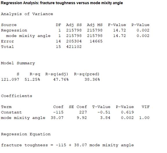
From the MINITAB output, the regression line is
Thus, the regression line for the variables fracture toughness
Interpretation:
The slope estimate implies an increase in fracture toughness by 38.07
The test hypotheses are given below:
Null hypothesis:
That is, there is no useful relationship between the variables fracture toughness
Alternative hypothesis:
That is, there is useful relationship between the variables fracture toughness
T-test statistic:
The test statistic is,
From the MINITAB output, the test statistic is 3.84 and the P-value is 0.002.
Thus, the value of test statistic is 3.84 and P-value is 0.002.
Level of significance:
Here, level of significance is not given.
So, the prior level of significance
Decision rule based on p-value:
If
If
Conclusion:
The P-value is 0.002 and
Here, P-value is less than the
That is
By the rejection rule, reject the null hypothesis.
Thus, there is enough evidence to conclude that the predictor variable mode-mixity angle is useful for predicting the value of the response variable fracture toughness.
b.
Test whether there is enough evidence to conclude that the change in fracture toughness associated with 1 degree increase in mode-mixity angle is greater than 50
b.
Answer to Problem 76SE
There is no sufficient evidence to conclude that the change in fracture toughness associated with 1 degree increase in mode-mixity angle is greater than 50
Explanation of Solution
Calculation:
From the MINITAB output obtained in part (a), the slope coefficient of the regression equation is
Here,
Claim:
Here, the claim is that the true average change in the fracture toughness associated with 1 degree increase in mode-mixity angle is greater than 50
The test hypotheses are given below:
Null hypothesis:
That is, the average change in the fracture toughness associated with 1 degree increase in mode-mixity angle is less than or equal to 50
Alternative hypothesis:
That is, the average change in the fracture toughness associated with 1 degree increase in mode-mixity angle is greater than 50
Test statistic:
The test statistic is,
Degrees of freedom:
The number of concrete beams that are sampled is
The degrees of freedom is,
Thus, the degree of freedom is 14.
Level of significance:
Here, level of significance is not given.
So, the prior level of significance
Critical value:
Software procedure:
Step by step procedure to obtain the critical value using the MINITAB software:
- Choose Graph > Probability Distribution Plot choose View Probability > OK.
- From Distribution, choose ‘t’ distribution and enter 14 as degrees of freedom.
- Click the Shaded Area tab.
- Choose Probability Value and Right Tail for the region of the curve to shade.
- Enter the Probability value as 0.05.
- Click OK.
Output using the MINITAB software is given below:
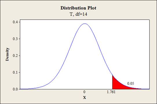
From the output, the critical value is 1.761.
Thus, the critical value is
From the MINITAB output obtained in part (a), the estimate of error standard deviation of slope coefficient is
Test statistic under null hypothesis:
Under the null hypothesis, the test statistic is obtained as follows:
Thus, the test statistic is -1.2026.
Decision criteria for the classical approach:
If
Conclusion:
Here, the test statistic is -1.2026 and critical value is 1.761.
The t statistic is less than the critical value.
That is,
Thus, the decision rule is, failed to reject the null hypothesis.
Hence, the average change in the fracture toughness associated with 1 degree increase in mode-mixity angle is less than or equal to 50
Therefore, there is no sufficient evidence to conclude that the change in fracture toughness associated with 1 degree increase in mode-mixity angle is greater than 50
c.
Explain whether the new observations of the variable mode-mixity angle give more precise estimate of slope coefficient than the actual observations.
c.
Answer to Problem 76SE
No, the new observations of the variable mode-mixity angle do not give more precise estimate of slope coefficient than the actual observations.
Explanation of Solution
Given info:
The data represents the new values of the variable mode-mixity angle, at which the response variable fracture toughness is predicted.
Calculation:
Confidence interval:
The general formula for the confidence interval for the slope of the regression line is,
Where,
The precision of the confidence interval increases with the decrease in the error standard deviation of the slope.
That is, the precision will be high for lower value of
Error sum of square: (SSE)
The variation in the observed values of the response variable that is not explained by the regression is defined as the regression sum of squares. The formula for error sum of square is
Estimate of error standard deviation of slope coefficient:
The general formula for the estimate of error standard deviation of slope coefficient is,
The defining formula for
Here, the estimate of error standard deviation of slope coefficient depends on the value of
The estimate of error standard deviation of slope coefficient decreases with the increase in the value of
The margin of error is product of critical value and standard error of the statistic. The higher width of the confidence interval indicates larger standard error of statistic. Hence, the margin of error also increases.
Therefore, the width of the confidence interval decreases with the decrease in value of error standard deviation. In other words it can be said that the precision decreases with the decrease in the value of
The value of
| 1 | 16.52 | 272.9104 |
| 2 | 17.53 | 307.3009 |
| 3 | 18.05 | 325.8025 |
| 4 | 18.05 | 325.8025 |
| 5 | 22.39 | 501.3121 |
| 6 | 23.89 | 570.7321 |
| 7 | 25.50 | 650.25 |
| 8 | 24.89 | 619.5121 |
| 9 | 23.48 | 551.3104 |
| 10 | 24.98 | 624.0004 |
| 11 | 25.55 | 652.8025 |
| 12 | 25.90 | 670.81 |
| 13 | 22.65 | 513.0225 |
| 14 | 23.69 | 561.2161 |
| 15 | 24.15 | 583.2225 |
| 16 | 24.45 | 597.8025 |
| Total |
Here,
Thus, the value of
Hence, the covariance is
The value of
| 1 | 16 | 256 |
| 2 | 16 | 256 |
| 3 | 18 | 324 |
| 4 | 18 | 324 |
| 5 | 20 | 400 |
| 6 | 20 | 400 |
| 7 | 20 | 400 |
| 8 | 20 | 400 |
| 9 | 22 | 484 |
| 10 | 22 | 484 |
| 11 | 22 | 484 |
| 12 | 22 | 484 |
| 13 | 24 | 576 |
| 14 | 24 | 576 |
| 15 | 26 | 676 |
| 16 | 26 | 676 |
| Total |
Here,
Thus, the value of
Hence, the covariance is
The value of
That is,
Hence, the estimate of error standard deviation of slope coefficient is lower for old observations.
Therefore, the precision is high for old observations.
Thus, the new observations of the variable mode-mixity angle do not give more precise estimate of slope coefficient than the actual observations.
d.
Find the
Find the prediction interval of fracture toughness for a single sandwich panel of 18 degrees mode-mixity angle.
Find the interval estimate for the true mean fracture toughness of all sandwich panels with 22 degrees mode-mixity angle.
Find the prediction interval of fracture toughness for a single sandwich panel of 22 degrees mode-mixity angle.
d.
Answer to Problem 76SE
The 95% specified confidence interval for the true mean fracture toughness of all sandwich panels with 18 degrees mode-mixity angle is
The 95% prediction interval of fracture toughness for a single sandwich panel with 18 degrees mode-mixity angle is
The 95% specified confidence interval for the true mean fracture toughness of all sandwich panels with 22 degrees mode-mixity angle is
The 95% prediction interval of fracture toughness for a single sandwich panel with 22 degrees mode-mixity angle is
Explanation of Solution
Calculation:
Here, the regression equation is
Expected fracture toughness when the mode-mixity angle is 18 degrees:
The expected fracture toughness with 18 degrees mode-mixity angle is obtained as follows:
Thus, the expected fracture toughness with 18 degrees mode-mixity angle is 570.26.
95% confidence interval of true mean fracture tough for an angle of 18 degrees:
The general formula for the
Where,
From the MINITAB output in part (a), the value of the standard error of the estimate is
The value of
| 1 | 16.52 | 272.9104 |
| 2 | 17.53 | 307.3009 |
| 3 | 18.05 | 325.8025 |
| 4 | 18.05 | 325.8025 |
| 5 | 22.39 | 501.3121 |
| 6 | 23.89 | 570.7321 |
| 7 | 25.50 | 650.25 |
| 8 | 24.89 | 619.5121 |
| 9 | 23.48 | 551.3104 |
| 10 | 24.98 | 624.0004 |
| 11 | 25.55 | 652.8025 |
| 12 | 25.90 | 670.81 |
| 13 | 22.65 | 513.0225 |
| 14 | 23.69 | 561.2161 |
| 15 | 24.15 | 583.2225 |
| 16 | 24.45 | 597.8025 |
| Total |
Here,
The mean mode-mixity angle is,
Thus, the mean mode-mixity angle is
Covariance term
Thus, the value of
Hence, the covariance is
Since, the level of confidence is not specified. The prior confidence level 95% can be used.
Critical value:
For 95% confidence level,
Degrees of freedom:
The sample size is
The degrees of freedom is,
From Table A.5 of the t-distribution in Appendix A, the critical value corresponding to the right tail area 0.025 and 14 degrees of freedom is 2.145.
Thus, the critical value is
The 95% confidence interval is,
Thus, the 95% specified confidence interval for the true mean fracture toughness of all sandwich panels with 18 degrees mode-mixity angle is
Interpretation:
There is 95% confident that, the true mean fracture toughness of all sandwich panels with 18 degrees mode-mixity angle lies between 453.6507 and 686.8693.
95% prediction interval of fracture tough for an angle of 18 degrees:
Prediction interval for a single future value:
Prediction interval is used to predict a single value of the focus variable that is to be observed at some future time. In other words it can be said that the prediction interval gives a single future value rather than estimating the mean value of the variable.
The general formula for
where
The 95% prediction interval is,
Thus, the 95% prediction interval of fracture toughness for a single sandwich panel with 18 degrees mode-mixity angle is
Interpretation:
For repeated samples, there is 95% confident that the fracture toughness for a single sandwich panel with 18 degrees mode-mixity angle lies between 285.5331 and 854.9569.
Expected fracture toughness when the mode-mixity angle is 22 degrees:
The expected fracture toughness with 22 degrees mode-mixity angle is obtained as follows:
Thus, the expected fracture toughness with 22 degrees mode-mixity angle is 722.54.
95% confidence interval of true mean fracture tough for an angle of 22 degrees:
The 95% confidence interval is,
Thus, the 95% specified confidence interval for the true mean fracture toughness of all sandwich panels with 22 degrees mode-mixity angle is
Interpretation:
There is 95% confident that, the true mean fracture toughness of all sandwich panels with 22 degrees mode-mixity angle lies between 656.3689 and 788.7111.
95% prediction interval of fracture tough for an angle of 22 degrees:
The 95% prediction interval is,
Thus, the 95% prediction interval of fracture toughness for a single sandwich panel with 22 degrees mode-mixity angle is
Interpretation:
For repeated samples, there is 95% confident that the fracture toughness for a single sandwich panel with 22 degrees mode-mixity angle lies between 454.491 and 990.589.
Want to see more full solutions like this?
Chapter 12 Solutions
PROB & STATS F/ ENGIN & SCI W/ACCESS


- A rural county presently uses Asphalt A to pave its highways, but is considering using themore expensive Asphalt B (which is reported to be more durable). The two types of asphaltare tested using 200m test strips on five different two-lane highways. On each test strip, arandomly selected lane was paved with Asphalt A and the lane in the opposing direction waspaved with Asphalt B. It has been determined that it is more economical to use Asphalt B ifthe length of time before resurfacing is required (i.e. longevity) is at least 2.5 years longer onaverage than that of Asphalt A. Assume that the longevity of each type of asphalt is normally distributed. Using a 2% significance level and assuming that the data for the two types of asphalt at eachtest strip can be paired, determine if Asphalt B lasts at least 2.5 years longer than Asphalt Aon average. Location 1 2 3 4 5Asphalt A 11.2 9.0 10.7 11.4 8.5Asphalt B 18.8 11.7 19.9 19.0 13.4arrow_forwardThe article “Withdrawal Strength of Threaded Nails” (D. Rammer, S. Winistorfer, and D. Bender, Journal of Structural Engineering 2001:442–449) describes an experiment comparing the ultimate withdrawal strengths (in N/mm) for several types of nails. For an annularly threaded nail with shank diameter 3.76 mm driven into spruce-pine-fir lumber, the ultimate withdrawal strength was modeled as lognormal with μ = 3.82 and σ = 0.219. For a helically threaded nail under the same conditions, the strength was modeled as lognormal with μ = 3.47 and σ = 0.272. a) What is the mean withdrawal strength for annularly threaded nails? b) What is the mean withdrawal strength for helically threaded nails? c) For which type of nail is it more probable that the withdrawal strength will be greater than 50 N/mm? d) What is the probability that a helically threaded nail will have a greater withdrawal strength than the median for annularly threaded nails? e) An experiment is performed in which withdrawal…arrow_forwardAn article in Knee Surgery, Sports Traumatology, Arthroscopy, "Arthroscopic meniscal repair with an absorbable screw: results and surgical technique," (2005, Vol. 13, pp. 273-279) cites a success rate of 1% for meniscal tears with a rim width of less than 3 mm, and a 1% success rate for tears from 3-6 mm. If you are unlucky enough to suffer a meniscal tear of less than 3 mm on your left knee, and one of width 3-6 mm on your right knee, what is the probability that you have exactly one successful surgery? assume surgieries are independent.arrow_forward
- In which situation cointegration test can be performed? Write down its null Also, refer the given table and interpret the results?arrow_forwardIn terms of the model parameters, state the null hypothesis that, after controlling for sales and roe, ros has no effect on CEO salary. State the alternative that better stock market performance increases a CEO’s salary.arrow_forwardIt has been shown that the fertilizer magnesium ammonium phosphate, Mg, NH4PO4, is an effective supplier of the nutrients necessary for plant growth. A study was conducted at George Mason University to determine a possible optimum level of fertilization, based on the enhanced vertical growth response of the chrysanthemums. Forty chrysanthemum seedlings were divided into four groups, each containing 10 plants. Each was planted in a similar pot containing a uniform growth medium. To each group of plants an increasing concentration of Mg,NH4PO4, measured in grams per bushel, was added: 50 g/bu, 100 g/bu, 200 g/bu, and 400g/bu. The sample means for each group was 15.34 cm, 17.16 cm, 18.3 cm, and 20.1 cm, respectively. Here SST = 758.035. (a) Construct the ANOVA table. (b) Use the Bonferroni correction to construct all g pairwise confidence intervals with t a df 2.792. What is a?arrow_forward
- The article in the ASCE Journal of Energy Engineering (1999, Vol. 125, pp.59-75) describes a study of the thermal inertia properties of autoclaved aerated concrete used as a building material. Five samples of the material were tested in a structure, and the average interior temperatures (°C) reported were as follows: 23.01, 22.22, 22.04, 22.62, and 22.59. Test that the average interior temperature is equal to 22.5°C using alpha (a) = 0.05. This problem is a test on what population parameter? What is the null and alternative hypothesis? What are the Significance level and type of test? What standardized test statistic will be used? What is the standard test statistic? What is the Statistical Decision? What is the statistical decision in the statement form?arrow_forwardAn observer at a busy bus stop did a 30-minute study of 3 buses. Given the following -Alight time =2 sec -Board time=3 sec -Door opening time =5 sec Determine the dwell time for the 3 busesarrow_forwardAn article in the Journal of Applied Polymer Science (Vol. 56, pp. 471–476, 1995) studied the effect of the mole ratio of sebacic acid on the intrinsic viscosity of copolyesters.- The data follows: Viscosity 0.45 0.2 0.34 0.58 0.7 0.57 0.55 0.44 Mole ratio 1 0.9 0.8 0.7 0.6 0.5 0.4 0.3 (a) Construct a scatter diagram of the data.arrow_forward
- Consider the accompanying data on flexural strength (MPa) for concrete beams of a certain type. 5.5 7.2 7.3 6.3 8.1 6.8 7.0 7.2 6.8 6.5 7.0 6.3 7.9 9.0 8.7 8.7 7.8 9.7 7.4 7.7 9.7 8.0 7.7 11.6 11.3 11.8 10.7 The data below give accompanying strength observations for cylinders. 6.6 5.8 7.8 7.1 7.2 9.2 6.6 8.3 7.0 8.4 7.3 8.1 7.4 8.5 8.9 9.8 9.7 14.1 12.6 11.3 Prior to obtaining data, denote the beam strengths by X1, . . . , Xm and the cylinder strengths by Y1, . . . , Yn. Suppose that the Xi's constitute a random sample from a distribution with mean μ1 and standard deviation σ1 and that the Yi's form a random sample (independent of the Xi's) from another distribution with mean μ2 and standard deviation σ2. Compute the estimated standard error. (Round your answer to three decimal places.) (c) Calculate a point estimate of the ratio σ1/σ2 of the two standard deviations. (Round your answer to three decimal places.) (d) Suppose a single beam and a single cylinder are…arrow_forwardConsider the accompanying data on flexural strength (MPa) for concrete beams of a certain type. 5.3 7.2 7.3 6.3 8.1 6.8 7.0 7.1 6.8 6.5 7.0 6.3 7.9 9.0 9.0 8.7 7.8 9.7 7.4 7.7 9.7 7.9 7.7 11.6 11.3 11.8 10.7 The data below give accompanying strength observations for cylinders. 6.8 5.8 7.8 7.1 7.2 9.2 6.6 8.3 7.0 9.0 7.6 8.1 7.4 8.5 8.9 9.8 9.7 14.1 12.6 11.8 Prior to obtaining data, denote the beam strengths by X1, . . . , Xm and the cylinder strengths by Y1, . . . , Yn. Suppose that the Xi's constitute a random sample from a distribution with mean ?1 and standard deviation ?1 and that the Yi's form a random sample (independent of the Xi's) from another distribution with mean ?2 and standard deviation ?2. (a) Calculate the estimate for the given data. (Round your answer to three decimal places.) (b) Use rules of variance to obtain an expression for the variance and standard deviation (standard error) of the estimator in part (a). V(X − Y) = V(X) + V(Y) =…arrow_forwardThe spike stature of the plants grown from the seeds of the porcine separates (Dactylis glomerata L) collected from the University campus and İbradı Eynif pasture are given below. In this plant, compare whether there is a difference between regions in terms of spike height. Virgo Height (cm) Data obtained from plants collected from university campus 5 6 8 7 8 6 5 5 4 6 6 Data obtained from plants collected from Eynif pasture 12 9 11 9 9 11 9 10 11 10 Note: Your results interpretation according to two different possibilities (Do it separately, assuming that it is 0.07 and 0.04).arrow_forward
 MATLAB: An Introduction with ApplicationsStatisticsISBN:9781119256830Author:Amos GilatPublisher:John Wiley & Sons Inc
 Probability and Statistics for Engineering and th...StatisticsISBN:9781305251809Author:Jay L. DevorePublisher:Cengage Learning
 Statistics for The Behavioral Sciences (MindTap C...StatisticsISBN:9781305504912Author:Frederick J Gravetter, Larry B. WallnauPublisher:Cengage Learning
 Elementary Statistics: Picturing the World (7th E...StatisticsISBN:9780134683416Author:Ron Larson, Betsy FarberPublisher:PEARSON
 The Basic Practice of StatisticsStatisticsISBN:9781319042578Author:David S. Moore, William I. Notz, Michael A. FlignerPublisher:W. H. Freeman
 Introduction to the Practice of StatisticsStatisticsISBN:9781319013387Author:David S. Moore, George P. McCabe, Bruce A. CraigPublisher:W. H. Freeman