Statistics for Business and Economics Plus MyLab Statistics with Pearson eText -- Title-Specific Access Card Package (13th Edition)
13th Edition
ISBN: 9780134763743
Author: James T. McClave, P. George Benson, Terry T Sincich
Publisher: PEARSON
expand_more
expand_more
format_list_bulleted
Concept explainers
Videos
Textbook Question
Chapter 12.6, Problem 12.53LM
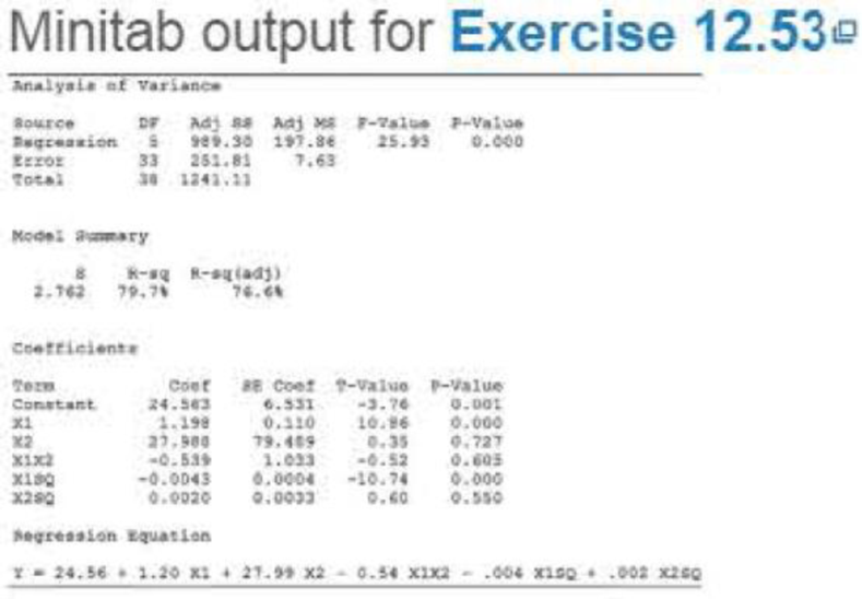
Minitab was used to fit the complete second-order model
E(y) = β0 + β1x1 + β2x2 + β3x1x2 + β4
to n = 39 data points. The printout is shown on the next page.
- a. Is there sufficient evidence to indicate that at least one of the parameters—β1, β2, β3, β4, and β5—is nonzero? Test using α =.05.
- b. Test H0 : β4 = 0 against Ha : β4 ≠ 0. Use α =.01.
- c. Test H0 : β5 = 0 against Ha : β4 ≠ 0. Use α =.01.
- d. Use graphs to explain the consequences of the tests in parts b and c.
Expert Solution & Answer
Want to see the full answer?
Check out a sample textbook solution
Students have asked these similar questions
In a typical multiple linear regression model where x1 and x2 are non-random
regressors, the expected value of the response variable y given x1 and x2 is denoted
by E(y | 2,, X2). Build a multiple linear regression model for E (y | *,, *2) such that the
value of E(y | x1, X2) may change as the value of x2 changes but the change in the
value of E(y | X1, X2) may differ in the value of x1 . How can such a potential difference
be tested and estimated statistically?
Consider the following regression model
Yt = β0 + β1 Ut + β2 Vt + β3 Wt + β4Xt + ∈t ,
where U, V, W, X and Y are economic variables observed from t = 1, . . . , 75, β0 , . . . , β4 are the model parameters and ∈t is the random disturbance term satisfying the classical assumptions. Ordinary Least Squares (OLS) is used to estimate the parameters, producing the following estimated model:
Yt = 1.115 + 0.790*Ut − 0.327*Vt + 0.763*Wt + 0.456*Xt
(0.405) (0.178) (0.088) (0.274) (0.017)
where standard errors are given in parentheses, the R-squared = 0.941, the Durbin-Watson statistic is DW = 1.907 and the residual sum of squares is RSS = 0.0757. In answering this question, use the 5% level of significance for any hypothesis tests that you are asked to perform, state clearly the null and al- ternative hypotheses that you are testing, the test statistics that you are using and interpret the decisions that you make.…
Consider the fitted values from a simple linear regression model with intercept: yˆ = 5 + 6x. Assume that the total number of observations is n = 302. In addition, the R-squared of the regression is R2 = 0.6 and Pn i=1(xi − x¯) 2 = 15, where ¯x is the sample mean of x. Under the classical Gauss-Markov assumptions, a) What is the standard error of the estimated slope coefficient?
Chapter 12 Solutions
Statistics for Business and Economics Plus MyLab Statistics with Pearson eText -- Title-Specific Access Card Package (13th Edition)
Ch. 12.3 - Write a first-order model relating E(y) to a. two...Ch. 12.3 - Minitab was used to fit the model E(y) = (0 + 1x1...Ch. 12.3 - Suppose you fit the multiple regression model y =0...Ch. 12.3 - Suppose you fit the first-order multiple...Ch. 12.3 - Prob. 12.5LMCh. 12.3 - Prob. 12.6LMCh. 12.3 - Prob. 12.7LMCh. 12.3 - If the analysis of variance F-test leads to the...Ch. 12.3 - Ambiance of 5-star hotels. Although invisible and...Ch. 12.3 - Forecasting movie revenues with Twitter. Refer to...
Ch. 12.3 - Accounting and Machiavellianism. Refer to the...Ch. 12.3 - Prob. 12.12ACBCh. 12.3 - Predicting elements in aluminum alloys. Aluminum...Ch. 12.3 - Novelty of a vacation destination. Many tourists...Ch. 12.3 - Arsenic in groundwater. Environmental Science ...Ch. 12.3 - Reality TV and cosmetic surgery. How much...Ch. 12.3 - Contamination from a plant's discharge. Refer to...Ch. 12.3 - Cooling method for gas turbines. Refer to the...Ch. 12.3 - Rankings of research universities. Refer to the...Ch. 12.3 - Bubble behavior in subcooled flow boiling. In...Ch. 12.3 - Prob. 12.22ACICh. 12.3 - Prob. 12.23ACACh. 12.3 - Prob. 12.24ACACh. 12.4 - Characteristics of lead users. Refer to the...Ch. 12.4 - Prob. 12.26ACBCh. 12.4 - Reality TV and cosmetic surgery. Refer to the Body...Ch. 12.4 - Chemical plant contamination. Refer to Exercise...Ch. 12.4 - Prob. 12.29ACBCh. 12.4 - Arsenic in groundwater. Refer to the Environmental...Ch. 12.4 - Prob. 12.32ACICh. 12.4 - Prob. 12.33ACICh. 12.4 - Boiler drum production. In a production facility,...Ch. 12.5 - Suppose the true relationship between E(y) and the...Ch. 12.5 - Suppose you fit the interaction model y = 0 + x1 +...Ch. 12.5 - Prob. 12.37LMCh. 12.5 - Tipping behavior in restaurants. Can food servers...Ch. 12.5 - Forecasting movie revenues with Twitter. Refer to...Ch. 12.5 - Prob. 12.41ACBCh. 12.5 - Prob. 12.42ACBCh. 12.5 - Reality TV and cosmetic surgery. Refer to the Body...Ch. 12.5 - Factors that impact an auditors judgment. A study...Ch. 12.5 - Service workers and customer relations. A study in...Ch. 12.5 - Bubble behavior in subcooled flow boiling. Refer...Ch. 12.5 - Arsenic in groundwater. Refer to the Environmental...Ch. 12.5 - Cooling method for gas turbines. Refer to the...Ch. 12.6 - Write a second-order model relating the mean of y,...Ch. 12.6 - Prob. 12.50LMCh. 12.6 - Prob. 12.51LMCh. 12.6 - Prob. 12.52LMCh. 12.6 - Minitab was used to fit the complete second-order...Ch. 12.6 - Personality traits and job performance. When...Ch. 12.6 - Going for it on fourth-down in the NFL. Refer to...Ch. 12.6 - Prob. 12.56ACBCh. 12.6 - Prob. 12.57ACBCh. 12.6 - Assertiveness and leadership. Management...Ch. 12.6 - Goal congruence in top management teams. Do chief...Ch. 12.6 - Prob. 12.60ACICh. 12.6 - Revenues of popular movies. The Internet Movie...Ch. 12.6 - Prob. 12.62ACICh. 12.6 - Prob. 12.63ACICh. 12.6 - Prob. 12.64ACICh. 12.6 - Prob. 12.65ACICh. 12.7 - Write a regression model relating the mean value...Ch. 12.7 - Prob. 12.67LMCh. 12.7 - Prob. 12.68LMCh. 12.7 - Prob. 12.69LMCh. 12.7 - Prob. 12.70ACBCh. 12.7 - Prob. 12.71ACBCh. 12.7 - Prob. 12.72ACBCh. 12.7 - Prob. 12.73ACBCh. 12.7 - Buy-side vs. sell-side analysts earnings...Ch. 12.7 - Prob. 12.75ACBCh. 12.7 - Charisma of top-level leaders. Refer to the...Ch. 12.7 - Corporate sustainability and firm characteristics....Ch. 12.7 - Homework assistance for accounting students. Refer...Ch. 12.7 - Improving driving performance while fatigued....Ch. 12.7 - Prob. 12.80ACACh. 12.7 - Banning controversial sports team sponsors. Refer...Ch. 12.8 - Consider a multiple regression model for a...Ch. 12.8 - Prob. 12.83LMCh. 12.8 - Consider the model: y = 0+ 1x1+ 2 x2+ 3 x3+...Ch. 12.8 - Consider the model:...Ch. 12.8 - Prob. 12.86LMCh. 12.8 - Reality TV and cosmetic surgery. Refer to the Body...Ch. 12.8 - Do blondes raise more funds? Refer to the Economic...Ch. 12.8 - Prob. 12.89ACBCh. 12.8 - Buy-side vs. sell-side analysts earnings...Ch. 12.8 - Workplace bullying and intention to leave....Ch. 12.8 - Agreeableness, gender, and wages. Do agreeable...Ch. 12.8 - Chemical plant contamination. Refer to Exercise...Ch. 12.8 - Prob. 12.94ACICh. 12.8 - Recently sold, single-family homes. The National...Ch. 12.8 - Charisma of top-level leaders Refer to the Academy...Ch. 12.9 - Determine which pairs of the following models are...Ch. 12.9 - Prob. 12.98LMCh. 12.9 - Prob. 12.99LMCh. 12.9 - Shared leadership in airplane crews. Refer to the...Ch. 12.9 - Buy-side vs. sell-side analysts earnings...Ch. 12.9 - Workplace bullying and intention to leave. Refer...Ch. 12.9 - Cooling method for gas turbines. Refer to the...Ch. 12.9 - Prob. 12.104ACBCh. 12.9 - Reality TV and cosmetic surgery. Refer to the Body...Ch. 12.9 - Study of supervisor-targeted aggression....Ch. 12.9 - Prob. 12.107ACICh. 12.9 - Recently sold, single-family homes. Refer to the...Ch. 12.9 - Prob. 12.109ACICh. 12.9 - Prob. 12.110ACACh. 12.10 - Prob. 12.111LMCh. 12.10 - Teacher pay and pupil performance. In Economic...Ch. 12.10 - Risk management performance. An article in the...Ch. 12.10 - Accuracy of software effort estimates....Ch. 12.10 - Diet of ducks bred for broiling. Corn is high in...Ch. 12.10 - Reality TV and cosmetic surgery. Refer to the Body...Ch. 12.10 - Prob. 12.117ACICh. 12.10 - Prob. 12.118ACICh. 12.10 - Prob. 12.119ACICh. 12.12 - Identify the problem(s) in each of the residual...Ch. 12.12 - Consider fitting the multiple regression model...Ch. 12.12 - Emotional intelligence and team performance. Refer...Ch. 12.12 - State casket sales restrictions. Some states...Ch. 12.12 - Personality traits and job performance. Refer to...Ch. 12.12 - Women in top management. Refer to the Journal of...Ch. 12.12 - Accuracy of software effort estimates. Refer to...Ch. 12.12 - Arsenic in groundwater. Refer to the Environmental...Ch. 12.12 - Reality TV and cosmetic surgery. Refer to the Body...Ch. 12.12 - Failure times of silicon wafer microchips. Refer...Ch. 12.12 - Bubble behavior in subcooled flow boiling. Refer...Ch. 12.12 - Banning controversial sports team sponsors. Refer...Ch. 12.12 - Cooling method for gas turbines. Refer to the...Ch. 12.12 - Agreeableness, gender, and wages. Refer to the...Ch. 12 - Suppose you have developed a regression model to...Ch. 12 - When a multiple regression model is used for...Ch. 12 - Suppose you fit the model y=0+1x1+2x12+3x2+4x1x2+...Ch. 12 - Prob. 12.137LMCh. 12 - Prob. 12.138LMCh. 12 - Prob. 12.139LMCh. 12 - Prob. 12.140LMCh. 12 - Prob. 12.141LMCh. 12 - Prob. 12.142LMCh. 12 - Prob. 12.143LMCh. 12 - Prob. 12.144LMCh. 12 - Comparing private and public college tuition....Ch. 12 - Prob. 12.146ACBCh. 12 - Prob. 12.147ACBCh. 12 - Highway crash data analysis. Researchers at...Ch. 12 - Prob. 12.149ACBCh. 12 - Mental health of a community. An article in the...Ch. 12 - Prob. 12.151ACBCh. 12 - Testing tires for wear. Underinflated or...Ch. 12 - Prob. 12.153ACBCh. 12 - Prob. 12.154ACBCh. 12 - Prob. 12.155ACBCh. 12 - Prob. 12.156ACBCh. 12 - Prob. 12.157ACBCh. 12 - Promotion of supermarket vegetables. A supermarket...Ch. 12 - Yield strength of steel alloy. Industrial...Ch. 12 - Prob. 12.160ACICh. 12 - Prob. 12.161ACICh. 12 - Improving Math SAT scores. Refer to the Chance...Ch. 12 - Prob. 12.163ACICh. 12 - Prob. 12.164ACICh. 12 - Prob. 12.165ACICh. 12 - Prob. 12.166ACICh. 12 - Sale prices of apartments. A Minneapolis,...Ch. 12 - Volatility of foreign stocks. The relationship...Ch. 12 - Prob. 12.169ACICh. 12 - Prob. 12.170ACICh. 12 - State casket sales restrictions Refer to the...Ch. 12 - Modeling monthly collision claims. A medium-sized...Ch. 12 - Developing a model for college GPA. Many colleges...
Knowledge Booster


Learn more about
Need a deep-dive on the concept behind this application? Look no further. Learn more about this topic, statistics and related others by exploring similar questions and additional content below.Similar questions
- In a multiple linear regression model with 3 predictor variables, what is the t-statistic for the hypothesis test of the null hypothesis that the coefficient of the second predictor variable is equal to 0, if the estimated coefficient is 0.5, the standard error of the estimate is 0.1, and the degrees of freedom is 15?arrow_forwardIn an instrumental variable regression model with one regressor, Xi, andone instrument, Zi, the regression of Xi onto Zi has R2 = 0.1 and n = 50.Is Zi a strong instrument? Would your answer change if R2 = 0.1 and n = 150?arrow_forwardAre the following statements true or false? Explain your answer.a. “An ordinary least squares regression of Y onto X will not be internallyvalid if Y is correlated with the error term.”b. “If the error term exhibits heteroskedasticity, then the estimates of Xwill always be biased.”arrow_forward
- An article in Biotechnology Progress [“Optimization of Conditions for Bacteriocin Extraction in PEG/Salt Aqueous Two-Phase Systems Using Statistical Experimental Designs” (2001, Vol. 17, pp. 366–368)] reported an experiment to investigate and optimize the extraction of nisin in aqueous two-phase systems (ATPS). Nisin recovery was the dependent variable (y). The two regressor variables were the concentration (%) of PEG 4000 (indicated as x1) and the concentration (%) of Na2SO4 (indicated as x2). The data is shown below. a) Find the fit parameters of the proposed model. b) Establish, by means of a hypothesis test, if the regression is significant. c) State, if the regression coefficients are significant. d) Evaluate R2 as well as R_adjusted^2. e) Construct and analyze the residual plot.arrow_forwardIn a laboratory experiment, data were gathered on the life span (y in months) of 33 rats, units of daily protein intake (x1), and whether or not agent x2 (a proposed life-extending agent) was added to the rats' diet (x2 = 0 if agent x2 was not added, and x2 = 1 if agent was added). From the results of the experiment, the following regression model was developed:ŷ = 36 + .8x1 − 1.7x2Also provided are SSR = 60 and SST = 180.The test statistic for testing the significance of the model is _____. a. 5.00 b. .50 c. .25 d. .33arrow_forwardContains 20 observations on the response variable y along with the predictor variables x and d. y x d 26 80 1 16 80 1 24 59 0 13 51 0 17 55 0 16 55 1 8 20 0 15 35 1 21 48 0 17 42 0 20 78 1 14 52 1 20 62 0 15 32 0 23 45 1 6 27 0 17 65 0 22 59 1 8 21 0 15 30 1 a. Estimate a regression model with the predictor variables x and d, and then extend it to also include the interaction variable xd. What is the estimated regression coefficient for the predictor variable x in both models? (Negative values should be indicated by a minus sign. Round your answers to 2 decimal places.) ) Model 1(No Interaction) = Model 2 (Interaction)= a-2. Use the preferred model to predict y. (Round coefficient estimates to at least 4 decimal places and final answers to 2 decimal places.) Predictor Variables Predicted Y x=15, d=0 ? x=15, d=1. ?arrow_forward
- The accompanying data file contains 40 observations on the response variable y along with the predictor variables x1 and x2. Use the holdout method to compare the predictability of the linear model with the exponential model using the first 30 observations for training and the remaining 10 observations for validation. y x1 x2 533.86 20 30 104.84 15 20 64.89 20 23 159.61 16 21 43.06 13 16 4.27 13 13 736.56 15 30 64.89 20 23 10.64 20 22 76.90 18 20 4.89 11 13 80.90 11 16 224.17 12 19 45.75 16 25 8.13 17 17 319.97 13 30 48.61 19 25 564.67 12 27 111.87 11 25 152.39 13 24 13.34 18 14 28.80 15 22 37.56 13 15 105.62 17 26 44.05 18 21 451.65 17 28 10.34 18 21 32.70 12 13 19.21 14 12 14.02 15 16 2.45 16 12 2.48 20 15 50.34 17 21 29.31 17 20 33.75 16 12 196.28 17 29 943.12 13 30 7.25 10 12 89.73 15 25 32.91 12 18 1. Use the training set to estimate Models 1 and 2. Note: Negative values should be indicated by a…arrow_forwardConsider a linear regression model where y represents the response variable and x and d are the predictor variables; d is a dummy variable assuming values 1 or 0. A model with x, d, and the interaction variable xd is estimated as ŷ= 5.20 + 1.60x + 1.40d + 0.20xd.a. Compute ŷ for x = 10 and d = 1. (Round your answer to 1 decimal place.) ŷ= b. Compute yˆy^ for x = 10 and d = 0. (Round your answer to 1 decimal place.) ŷ=arrow_forwardThe accompanying data file contains 40 observations on the response variable y along with the predictor variables x and d. Consider two linear regression models where Model 1 uses the variables x and d and Model 2 extends the model by including the interaction variable xd. Use the holdout method to compare the predictability of the models using the first 30 observations for training and the remaining 10 observations for validation. y x d 70 11 1 102 19 1 76 12 1 83 14 1 61 17 0 62 13 0 67 20 0 98 16 1 84 11 1 101 15 1 51 16 0 108 16 1 32 13 0 71 15 1 101 17 1 90 15 1 112 19 1 88 13 1 110 18 1 95 17 1 44 14 0 51 19 0 112 17 1 113 17 1 52 13 0 61 10 1 100 16 1 78 14 1 90 16 1 57 16 0 59 15 0 53 15 0 119 19 1 109 18 1 68 11 0 104 19 1 45 18 0 67 17 0 65 15 0 74 14 1 1. Use the training set to estimate Models 1 and 2. Note: Negative values should be indicated by a minus sign. Round your answers to 2…arrow_forward
- In a data set with 12 observations, you try fitting two regression models. The esti-mated models are summarized as: Model 1: Y(hat) =3.5 + 2x; SSR= 5, and SSE= 10;Model 2: Y(hat) =3.0 + 1.5x + 0.4^2; SSR=23, and SSE=7 (a) Calculate R2 for both models. b. for both models test the null hypothesis that all the regression coefficients other than the intercept are 0.arrow_forwardConsider the following two a.m. peak work trip generation models, estimated by household linear regression: T = 0.62 + 3.1 X1 + 1.4 X2 R2= 0.590 (2.3) (7.1) (5.9) T = 0.01 + 2.4 X1 + 1.2 Z1 + 4.0 Z2 R2= 0.598 (0.8) (4.2) (1.7) (3.1) X1 = number of workers in the household X2 = number of cars in the household, Z1 is a dummy variable which takes the value 1 if the household has one car, Z2 is a dummy variable which takes the value 1 if the household has two or more cars. Compare the two models and choose the best. If a zone has 1000 households, of which 50% have no car, 35% have one car, and the rest have exactly two cars, estimate the total number of trips generated by this zone. Use the preferred trip generation model and assume that each household has an average of two workersarrow_forwardThe following table shows students’ test scores on the first two tests in an introductory physics class. Physics Test Scores First test, x 7373 6161 6969 4242 8888 8787 4242 4444 4040 4848 6868 6464 Second test, y 7474 6262 6262 4343 7878 6969 3838 4343 3030 4848 6666 5454 Step 1 of 2 : Find an equation of the least-squares regression line. Round your answer to three decimal places, if necessary. Step 2 of 2 : If a sudent scored a 75 on his first paper, make a prediction for his score on the second test. Assume the regression equation is appropriate for prediction. Round your answer to two decimal places, if necessary.arrow_forward
arrow_back_ios
SEE MORE QUESTIONS
arrow_forward_ios
Recommended textbooks for you
 MATLAB: An Introduction with ApplicationsStatisticsISBN:9781119256830Author:Amos GilatPublisher:John Wiley & Sons Inc
 Probability and Statistics for Engineering and th...StatisticsISBN:9781305251809Author:Jay L. DevorePublisher:Cengage Learning
 Statistics for The Behavioral Sciences (MindTap C...StatisticsISBN:9781305504912Author:Frederick J Gravetter, Larry B. WallnauPublisher:Cengage Learning
 Elementary Statistics: Picturing the World (7th E...StatisticsISBN:9780134683416Author:Ron Larson, Betsy FarberPublisher:PEARSON
 The Basic Practice of StatisticsStatisticsISBN:9781319042578Author:David S. Moore, William I. Notz, Michael A. FlignerPublisher:W. H. Freeman
 Introduction to the Practice of StatisticsStatisticsISBN:9781319013387Author:David S. Moore, George P. McCabe, Bruce A. CraigPublisher:W. H. Freeman
MATLAB: An Introduction with Applications
Statistics
ISBN:9781119256830
Author:Amos Gilat
Publisher:John Wiley & Sons Inc
Probability and Statistics for Engineering and th...
Statistics
ISBN:9781305251809
Author:Jay L. Devore
Publisher:Cengage Learning
Statistics for The Behavioral Sciences (MindTap C...
Statistics
ISBN:9781305504912
Author:Frederick J Gravetter, Larry B. Wallnau
Publisher:Cengage Learning
Elementary Statistics: Picturing the World (7th E...
Statistics
ISBN:9780134683416
Author:Ron Larson, Betsy Farber
Publisher:PEARSON
The Basic Practice of Statistics
Statistics
ISBN:9781319042578
Author:David S. Moore, William I. Notz, Michael A. Fligner
Publisher:W. H. Freeman
Introduction to the Practice of Statistics
Statistics
ISBN:9781319013387
Author:David S. Moore, George P. McCabe, Bruce A. Craig
Publisher:W. H. Freeman
Statistics 4.1 Point Estimators; Author: Dr. Jack L. Jackson II;https://www.youtube.com/watch?v=2MrI0J8XCEE;License: Standard YouTube License, CC-BY
Statistics 101: Point Estimators; Author: Brandon Foltz;https://www.youtube.com/watch?v=4v41z3HwLaM;License: Standard YouTube License, CC-BY
Central limit theorem; Author: 365 Data Science;https://www.youtube.com/watch?v=b5xQmk9veZ4;License: Standard YouTube License, CC-BY
Point Estimate Definition & Example; Author: Prof. Essa;https://www.youtube.com/watch?v=OTVwtvQmSn0;License: Standard Youtube License
Point Estimation; Author: Vamsidhar Ambatipudi;https://www.youtube.com/watch?v=flqhlM2bZWc;License: Standard Youtube License