Concept explainers
Videos
a.
Construct a
a.
Answer to Problem 48CE
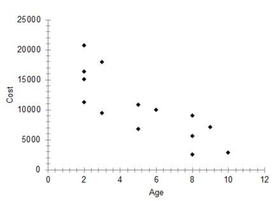
The scatter diagram of the data is as follows:
Explanation of Solution
It is given that ‘Estimated cost’ is the dependent variable.
Step-by-step procedure to obtain the scatterplot using the MegaStat software:
- In an EXCEL sheet enter the data values of x and y.
- Go to Add-Ins > MegaStat >
Correlation /Regression > Scatterplot. - Enter horizontal axis as $B$1:$B$15 and vertical axis as $A$1:$A$15.
- Click on OK.
From the scatterplot of the data, it indicates an inverse relationship.
b.
Find the
b.
Answer to Problem 48CE
The correlation coefficient is –0.822.
Explanation of Solution
Step-by-step procedure to obtain the correlation coefficient using the MegaStat software:
- In an EXCEL sheet enter the data values of x and y.
- Go to Add-Ins > MegaStat > Correlation/Regression > Correlation matrix.
- Enter Input
Range as $A$1:$B$15. - Click on OK.
Output obtained using the MegaStat is given as follows:
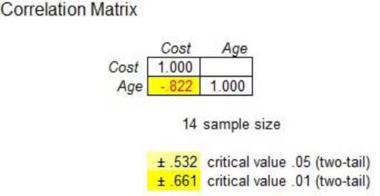
The correlation coefficient is –0.822. Since the correlation coefficient is negative and close to –1, there is a strong
c.
Interpret the slope of the regression equation.
c.
Explanation of Solution
The estimated regression equation is
The interpretation is that for each unit added to age, there is a decrease of $1,534 in cost.
d.
Estimate the cost of a five-year-old car.
d.
Answer to Problem 48CE
The estimated value of cost of a five-year-old car is $10,688.
Explanation of Solution
Substitute x as 5 in the regression equation.
Thus, the estimated value of cost of a five-year-old car is $10,688.
e.
Explain the given portion of the software output.
e.
Explanation of Solution
From the output p-value corresponding to the variable age is 0. That is, the p-value is less than any common level of significance. Thus, the variable age is significant.
f.
Test whether the slope is significant or not.
Interpret the result.
Check whether there is any significant relationship between the two variables.
f.
Answer to Problem 48CE
There is sufficient evidence to conclude that the slope of the regression line is different from zero at the 10% level of significance.
Explanation of Solution
It is given that the regression equation is
From the regression equation, the estimated slope of the regression line is
Let
The given test hypotheses are as follows:
Null hypothesis:
That is, the slope of the regression line is equal to zero.
Alternate hypothesis:
That is, the slope of the regression line is not equal to zero.
It is given that the level of significance is 0.10.
The standard error of
Test statistic:
The t-test statistic is as follows:
Where,
Thus, the following is obtained:
Here, the sample size is
Critical value:
Software procedure:
Step-by-step software procedure to obtain the critical value
- Open an EXCEL file.
- In cell A1, enter the formula “=T.INV(0.05,12)”.
Output obtained using the EXCEL is given as follows:
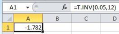
From the EXCEL output, the critical value is –1.782 (
Decision based on critical value:
Reject the null hypothesis, if
Conclusion:
The t-calculated value is 5.01 and the critical value is 1.782.
That is,
Thus, the null hypothesis is rejected.
Hence, there is sufficient evidence to conclude that the slope of the regression line is different from zero at the 10% level of significance.
Since the slope of the regression line is different from zero, there is a relationship between age and cost.
Want to see more full solutions like this?
Chapter 13 Solutions
EBK STATISTICAL TECHNIQUES IN BUSINESS


- Life Expectancy The following table shows the average life expectancy, in years, of a child born in the given year42 Life expectancy 2005 77.6 2007 78.1 2009 78.5 2011 78.7 2013 78.8 a. Find the equation of the regression line, and explain the meaning of its slope. b. Plot the data points and the regression line. c. Explain in practical terms the meaning of the slope of the regression line. d. Based on the trend of the regression line, what do you predict as the life expectancy of a child born in 2019? e. Based on the trend of the regression line, what do you predict as the life expectancy of a child born in 1580?2300arrow_forwardThe ordered pairs below give the median sales prices y (in thousands of dollars) of new homes sold in a neighborhood from 2009 through 2016. (2009, 179.4) (2011, 191.0) (2013, 202.6) (2015, 214.9) (2010, 185.4) (2012, 196.7) (2014, 208.7) (2016, 221.4) A linear model that approximates the data is y=5.96t+125.5,9t16, where t represents the year, with t=9 corresponding to 2009. Plot the actual data and the model on the same graph. How closely does the model represent the data?arrow_forwardDemand for Candy Bars In this problem you will determine a linear demand equation that describes the demand for candy bars in your class. Survey your classmates to determine what price they would be willing to pay for a candy bar. Your survey form might look like the sample to the left. a Make a table of the number of respondents who answered yes at each price level. b Make a scatter plot of your data. c Find and graph the regression line y=mp+b, which gives the number of respondents y who would buy a candy bar if the price were p cents. This is the demand equation. Why is the slope m negative? d What is the p-intercept of the demand equation? What does this intercept tell you about pricing candy bars? Would you buy a candy bar from the vending machine in the hallway if the price is as indicated. Price Yes or No 50 75 1.00 1.25 1.50 1.75 2.00arrow_forward
 Functions and Change: A Modeling Approach to Coll...AlgebraISBN:9781337111348Author:Bruce Crauder, Benny Evans, Alan NoellPublisher:Cengage Learning
 Glencoe Algebra 1, Student Edition, 9780079039897...AlgebraISBN:9780079039897Author:CarterPublisher:McGraw Hill
 Algebra and Trigonometry (MindTap Course List)AlgebraISBN:9781305071742Author:James Stewart, Lothar Redlin, Saleem WatsonPublisher:Cengage Learning
 Big Ideas Math A Bridge To Success Algebra 1: Stu...AlgebraISBN:9781680331141Author:HOUGHTON MIFFLIN HARCOURTPublisher:Houghton Mifflin Harcourt