
Concept explainers
Videos
(a)
To find: The means for each species by water combination and plot these means.
(a)
Answer to Problem 51E
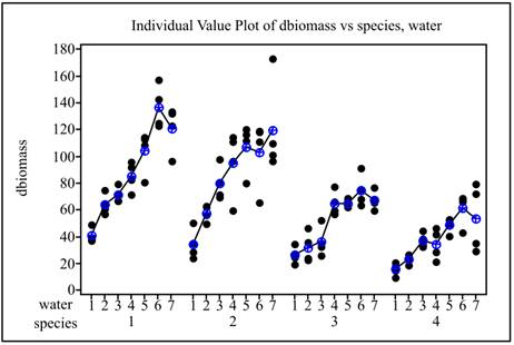
Solution: For Fresh biomass, the first three means for Species-1 are 109.1, 165.1, and 168.82. The first three means for Species-2 are 116.4, 156.8, and 254.88. The first three means for Species-3 are 55.60, 78.9, and 90.3. The first three means for Species-4 are 35.13, 58.33, and 94.54.
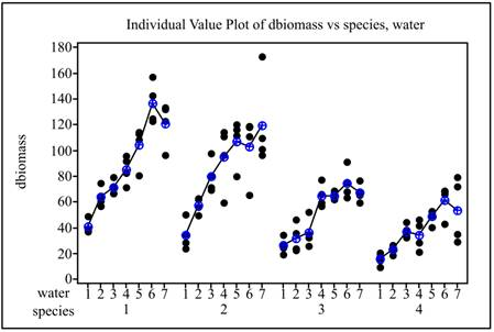
For Dry biomass, the first three means for Species-1 are 40.56, 63.86, and 71.00. The first three means for Species-2 are 34.50, 57.36, and 79.60. The first three means for Species-3 are 26.25, 31.87, and 36.24. The first three means for Species-4 are 15.53, 23.29, and 37.05.
Explanation of Solution
Calculation: To obtain the means for the response variable Fresh biomass, Minitab is used. The steps to be followed are:
Step 1: Go to the Minitab worksheet.
Step 2: Go to Stat
Step 3: Enter the variable ‘Fresh biomass’ in the ‘Variable’ option.
Step 4: Enter the variables ‘Species and Water’ in the ‘By Variable’ option.
Step 5: Go to statistics and select ‘Mean.
Step 6: Go to graph and select Individual value plot’.
Step 7: Click Ok.
The obtained result shows the means for each species by water level. Here, few of them are given: The first three means for Species-1 are 109.1, 165.1, and 168.82. The first three means for Species-2 are 116.4, 156.8, and 254.88. The first three means for species-3 are 55.60, 78.9, and 90.3. The first three means for Species-4 are 35.13, 58.33, and 94.54. The obtained graph is given below:
To obtain the means for the response variable Dry biomass, Minitab is used. The steps to be followed are:
Step 1: Go to the Minitab worksheet.
Step 2: Go to Stat
Step 3: Enter the variable ‘Dry biomass’ in the ‘Variable’ option.
Step 4: Enter the variables ‘Species and Water’ in the ‘By Variable’ option.
Step 5: Go to statistics and select ‘Mean.
Step 6: Go to graph and select Individual value plot’.
Step 7: Click Ok.
The obtained result shows the means for each species by water level. Here, few of them are given: The first three means for Species-1 are 40.56, 63.86, and 71.00. The first three means for Species-2 are 34.50, 57.36, and 79.60. The first three means for species-3 are 26.25, 31.87, and 36.24. The first three means for Species-4 are 15.53, 23.29, and 37.05. The obtained graph is given below:
(b)
To find: The standard deviation for each species by water combination and plot these means.
(b)
Answer to Problem 51E
Solution: For Fresh biomass, the first three standard deviations for Species-1 are 20.9, 29.1, and 18.87. The first three standard deviations for Species-2 are 29.3, 46.9, and 13.94. The first three standard deviations for Species-3 are 13.20, 29.5, and 28.3. The first three standard deviations for Species-4 are 11.63, 6.79, and 13.93.
For Dry biomass, the first three standard deviations for Species-1 are 5.58, 7.51, and 6.03. The first three standard deviations for Species-2 are 11.61, 6.15, and 13.09. The first three standard deviations for Species-3 are 6.43, 11.32, and 11.27. The first three standard deviations for Species-4 are 4.89, 3.33, and 5.19.
Explanation of Solution
Calculation: To obtain the means for Fresh biomass, Minitab is used. The steps to be followed are:
Step 1: Go to the Minitab worksheet.
Step 2: Go to Stat
Step 3: Enter the variable ‘Fresh biomass’ in the ‘Variable’ option.
Step 4: Enter the variables ‘Species and Water’ in the ‘By Variable’ option.
Step 5: Go to statistics and select ‘Standard deviation’.
Step 6: Click Ok.
The obtained result shows the means for each species by water level. Here, few of them are given: The first three standard deviations for Species-1 are 20.9, 29.1, and 18.87. The first three standard deviations for Species-2 are 29.3, 46.9, and 13.94. The first three standard deviations for species-3 are 13.20, 29.5, and 28.3. The first three standard deviations for Species-4 are 11.63, 6.79, and 13.93.
To obtain the means for Dry biomass, Minitab is used. The steps to be followed are:
Step 1: Go to the Minitab worksheet.
Step 2: Go to Stat
Step 3: Enter the variable ‘Dry biomass’ in the ‘Variable’ option.
Step 4: Enter the variables ‘Species and Water’ in the ‘By Variable’ option.
Step 5: Go to statistics and select ‘Standard deviation’.
Step 6: Click Ok.
The obtained result shows the means for each species by water level. Here, few of them are given: The first three standard deviations for Species-1 are 5.58, 7.51, and 6.03. The first three standard deviations for Species-2 are 11.61, 6.15, and 13.09. The first three standard deviations for species-3 are 6.43, 11.32, and 11.27. The first three standard deviations for Species-4 are 4.89, 3.33, and 5.19
The highest SD from the Fresh biomass data is 108.01 and the lowest SD is 6.79. Thus,
The highest SD from the Dry biomass data is 35.76 and the lowest SD is 3.12. Thus,
Hence, it is reasonable to pool the standard deviation.
(c)
To test: A two-way ANOVA for Fresh biomass and Dry biomass
(c)
Answer to Problem 51E
Solution: A two-way ANOVA for Fresh biomass is provided below:
Source of Variation |
Degree of freedom |
Sum of squares |
Mean sum of squares |
F- value |
P- value |
Species |
3 |
458295 |
152765 |
81.45 |
0.000 |
Water |
6 |
491948 |
81991 |
43.71 |
0.000 |
Interaction |
18 |
60334 |
3352 |
1.79 |
0.040 |
Error |
84 |
157551 |
1876 |
||
Total |
111 |
1168129 |
A two-way ANOVA for Dry biomass is provided below:
Source of Variation |
Degree of freedom |
Sum of squares |
Mean sum of squares |
F- value |
P- value |
Species |
3 |
50524 |
16841.3 |
79.93 |
0.000 |
Water |
6 |
56624 |
9437.3 |
44.79 |
0.000 |
Interaction |
18 |
8419 |
467.7 |
2.22 |
0.008 |
Error |
84 |
17698 |
219.7 |
||
Total |
111 |
133265 |
Explanation of Solution
Calculation: To perform a Two-way ANOVA for Fresh biomass, Minitab is used. The steps to be followed are:
Step 1: Go to the Minitab worksheet.
Step 2: Go to Stat
Step 3: Enter the variable ‘Fresh biomass’ in the ‘Response’ option.
Step 4: Enter the variables ‘Species’ in the ‘Row Factor and ‘Water’ in the Column Factor’.
Step 5: Click Ok.
The obtained results are provided below:
Source of Variation |
Degree of freedom |
Sum of squares |
Mean sum of squares |
F- value |
P- value |
Species |
3 |
458295 |
152765 |
81.45 |
0.000 |
Water |
6 |
491948 |
81991 |
43.71 |
0.000 |
Interaction |
18 |
60334 |
3352 |
1.79 |
0.040 |
Error |
84 |
157551 |
1876 |
||
Total |
111 |
1168129 |
To perform a Two-way ANOVA for Dry biomass, Minitab is used. The steps to be followed are:
Step 1: Go to the Minitab worksheet.
Step 2: Go to Stat
Step 3: Enter the variable ‘Dry biomass’ in the ‘Response’ option.
Step 4: Enter the variables ‘Species’ in the ‘Row Factor and ‘Water’ in the Column Factor’.
Step 5: Click Ok.
The obtained results are provided below:
Source of Variation |
Degree of freedom |
Sum of squares |
Mean sum of squares |
F- value |
P- value |
Species |
3 |
50524 |
16841.3 |
79.93 |
0.000 |
Water |
6 |
56624 |
9437.3 |
44.79 |
0.000 |
Interaction |
18 |
8419 |
467.7 |
2.22 |
0.008 |
Error |
84 |
17698 |
219.7 |
||
Total |
111 |
133265 |
Conclusion: From ANOVA table above, for both Fresh biomass and Dry biomass, main effects and interaction are significant. The interaction for Fresh biomass and Dry biomass has the P-value 0.04 and 0.008, respectively.
Want to see more full solutions like this?
Chapter 13 Solutions
Introduction to the Practice of Statistics


 MATLAB: An Introduction with ApplicationsStatisticsISBN:9781119256830Author:Amos GilatPublisher:John Wiley & Sons Inc
 Probability and Statistics for Engineering and th...StatisticsISBN:9781305251809Author:Jay L. DevorePublisher:Cengage Learning
 Statistics for The Behavioral Sciences (MindTap C...StatisticsISBN:9781305504912Author:Frederick J Gravetter, Larry B. WallnauPublisher:Cengage Learning
 Elementary Statistics: Picturing the World (7th E...StatisticsISBN:9780134683416Author:Ron Larson, Betsy FarberPublisher:PEARSON
 The Basic Practice of StatisticsStatisticsISBN:9781319042578Author:David S. Moore, William I. Notz, Michael A. FlignerPublisher:W. H. Freeman
 Introduction to the Practice of StatisticsStatisticsISBN:9781319013387Author:David S. Moore, George P. McCabe, Bruce A. CraigPublisher:W. H. Freeman