Concept explainers
Videos
(a)
To find: Inter
(a)
Answer to Problem 66E
Solution: The Inter
Explanation of Solution
Calculation: The Inter Quartile Range
Follow the steps given below:
Step 1: Enter the data in a Minitab worksheet.
Step 2: Go to Stat and select basic statistics.
Step 3: Then select Display
Step 4: Then click on Statistics tab and tick mark the option against Interquartile Range and click on OK twice.
From the Minitab output the Inter Quartile Range
Interpretation: The Inter Quartile Range
(b)
To find: The outliers using
(b)
Answer to Problem 66E
Solution: There are no outliers in the provided data. Any value above 77.48 or below 23.32 would be considered outliers as they are upper whisker and lower whisker, respectively. There is no value above or below those numbers respectively.
Explanation of Solution
Calculation: To obtain the value of first and third quartile, follow the steps given below in Minitab,
Step 1: Enter the data in a Minitab worksheet.
Step 2: Go to Stat and select basic statistics.
Step 3: Then select Display Descriptive Statistics. Enter the name of the column containing the Reflectance data in the variables textbox.
Step 4: Then click on Statistics tab and tick mark the option against first quartile and third quartile and click on OK twice.
The value of
The formula for upper whisker is,
Where
The formula for lower whisker is,
where
Upper whisker of boxplot is found to be 77.48, so any values above 77.48 would be considered outliers. There is no value that is either above upper whisker or below lower whisker, so there is no outlier.
Interpretation: Outliers refers to those data points that lie either above upper whisker or below lower whisker in boxplot. From the calculations done above, it is clear that the data does not contain any outlier.
(c)
To graph: A boxplot of the provided data and describe the distribution using it.
(c)
Explanation of Solution
Graph: Follow the steps given below to obtain the boxplot:
Step 1: Enter the data into a Minitab worksheet.
Step 2: Go to ‘Graph’ and click on ‘Boxplot’.
Step 3: In the dialogue box that appears select ‘Simple’ and click OK.
Step 4: Next enter the name of the column containing the data of reflectance of smolts in the filed marked as ‘Graph variables’ and click on OK.
The boxplot is obtained as shown below,
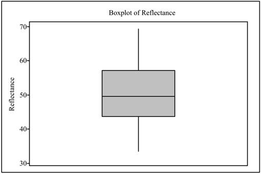
Interpretation: The boxplot is generally preferred to describe data set having unsymmetrical distribution. The boxplot shows First quartile, Median, and Third quartile. The boxplot of the data represents there are no outliers in the data.
(d)
To graph: A modified boxplot and describes the distribution using it.
(d)
Explanation of Solution
Graph: Follow the steps given below to obtain the modified boxplot:
Step 1: Enter the data into a Minitab worksheet.
Step 2: Go to ‘Graph’ and click on ‘Boxplot’.
Step 3: In the dialogue box that appears select ‘Simple’ and click OK.
Step 4: Next enter the name of the column containing the data of reflectance of smolts in the filed marked as ‘Graph variables’ and click on OK.
The boxplot is obtained as shown below,
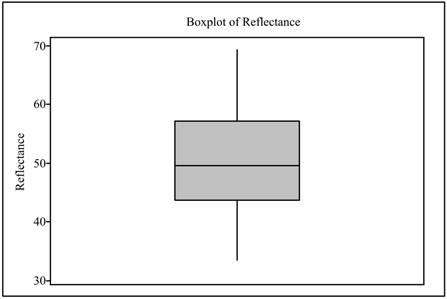
Interpretation: The modified boxplot is generally used to display data graphically when the distribution of data is unsymmetrical and skewed as it can clearly show outliers. In the above modified boxplot, there is no outlier, which indicates that the data distribution is symmetrical.
(e)
To graph: A stem plot of the provided data.
(e)
Answer to Problem 66E
Solution: The stemplot of the data is shown below:
Explanation of Solution
Graph:
Follow the steps given below to obtain the stemplot:
Step 1: Enter the provided data in a Minitab worksheet.
Step 2: Go to Graph and select stem and leaves.
Step 3: Enter the name of the column containing the provided data in the Graph variables textbox and click on OK.
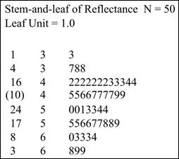
The obtained stem plot is displayed below,
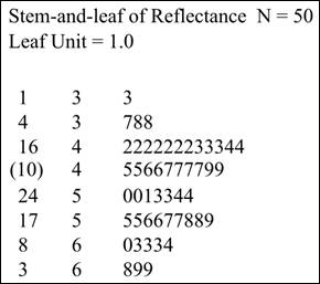
Interpretation: The stemplot of data is generally drawn when size of data is somewhat small and all the data values are positive. The graph shows all the data values on stemplot. In the stemplot shown above there is no outliers and therefore, it indicates that the distribution of the data is symmetrical.
(f)
To find: The Boxplot, Modified boxplot, and stemplot and their advantages and disadvantages.
(f)
Answer to Problem 66E
Solution: In boxplot, data is displayed based on five-number summary, which includes Minimum, Maximum, First quartile, Third Quartile, and Median. In Modified boxplot, also data is displayed based on five-number summary, but it also shows outliers. In stemplot, data values are arranged in stem consisting of all digits except right most and leaves contain final digit. Advantages of boxplots is that it is suitable for large unsymmetrical data while advantages of stemplot is that it shows all numerical value of data on graph itself. Disadvantage of Boxplot is that it is not suitable for unsymmetrical data and it does not retain exact numerical values while disadvantage of stemplot is that it is used only for positive numbers only and if data size is small.
Explanation of Solution
The comparison of Boxplot, Modified boxplot, and stemplot is shown below:
Boxplot |
Modified Boxplot |
Stemplot |
|
Description |
It displays data based on |
It displays data based on five number summary including Minimum, Maximum, First quartile, Third Quartile and Median. |
In stemplot data values are arranged in stem consisting of all digits except right most digit and leaves contain final digit |
Advantages |
1. It displays five number summary graphically. 2. It is suitable for unsymmetrical data. 3. It can handle large data set. |
1. It displays five number summary. 2. It is suitable for unsymmetrical data which is skewed. 3. It shows outliers clearly. |
1. It can display both symmetrical and unsymmetrical data graphically. 2. It can indicate outliers also. 3. It displays all numerical values of data on stemplot. |
Disadvantages |
1. It is not suitable for data set having symmetrical distribution. 2. It does not display outliers on graph. |
1. It is not suitable for data set having symmetrical distribution. |
1. It is not suitable if data size is very large. 2. It is not used for negative numbers. |
Interpretation: There are various ways to display data graphically, Boxplot is suitable for unsymmetrical data which are skewed, it can handle large data set as well, it shows five-number summary and displays Maximum, Minimum, first quartile, third quartile, and median, and also shows outliers. Stemplot plot is used if data size is small and greater than 0.
Want to see more full solutions like this?
Chapter 1 Solutions
Introduction to the Practice of Statistics: w/CrunchIt/EESEE Access Card


 MATLAB: An Introduction with ApplicationsStatisticsISBN:9781119256830Author:Amos GilatPublisher:John Wiley & Sons Inc
 Probability and Statistics for Engineering and th...StatisticsISBN:9781305251809Author:Jay L. DevorePublisher:Cengage Learning
 Statistics for The Behavioral Sciences (MindTap C...StatisticsISBN:9781305504912Author:Frederick J Gravetter, Larry B. WallnauPublisher:Cengage Learning
 Elementary Statistics: Picturing the World (7th E...StatisticsISBN:9780134683416Author:Ron Larson, Betsy FarberPublisher:PEARSON
 The Basic Practice of StatisticsStatisticsISBN:9781319042578Author:David S. Moore, William I. Notz, Michael A. FlignerPublisher:W. H. Freeman
 Introduction to the Practice of StatisticsStatisticsISBN:9781319013387Author:David S. Moore, George P. McCabe, Bruce A. CraigPublisher:W. H. Freeman